Mechanism Design
Jan Boone
jan.boone.uvt@gmail.com
Table of Contents
Introduction
What is mechanism design?
- We will consider situations where a principal wants an agent to do something
- Agent has private information that the principal cannot observe
- in optimal tax problem: government cannot observe my productivity
- in monopoly problem: monopolist cannot observe my valuation of the good
- government regulating NS cannot observe costs of operating a railway track
- ministry of health trying to limit health care expenditure cannot observe quality of hospitals, severity of patients
- government selling telecom licenses cannot observe utility that consumers will enjoy from these or the costs of operating such networks
- Agent’s private information gives him (bargaining/market) power and he can extract rents from the principal
- Principal wants to design a way to get the desired action from the agent at the lowest cost
- Instead of focusing on examples (like linear tax scheme, quadratic tax etc.), principal asks the agent directly what his type is
- And makes sure that the agent will reveal his type to her truthfully
- This is true for any mechanism that you can think of and –in fact– far easier to analyze
- Mechanism design gives you the tools to analyze situations like this
Why is this useful?
- It turns out to be analytically more convenient!
- It separates the optimal outcome from the way you would like to implement this outcome
- You get the optimal overall solution; not, say, the optimal linear solution
- It forces you to think about the things that really matter:
- what is the principal’s objective function?
- how can agents deviate (incentive compatibility)
- do agents want to participate (individual rationality)
- how to trade off efficiency and rent extraction
Optimal taxation (2 types)
Without mechanism design
- Consider utility function \(u(c)-n\) where \(c\) denotes consumption and \(n\) work effort
- \(u'(c)>0\)
- Decreasing marginal utility \(u''(c)<0\)
- There are two types of workers: low productivity \(w^l\) (fraction \(\phi\) of the population) and high productivity \(w^h>w^l\) (\(1-\phi\))
- Government cannot observe type \(w\) nor effort \(n\)
- Government only observes gross income \(y = w n\)
- At first sight, one would try to find a tax function \(T(y)\) to maximize (some) government objective
- Worker then solves
- First order condition
- Second order condition: oops?
- That is why we need mechanism design
With mechanism design
- Revelation principle: any mechanism that you can think of, can be described as “ask worker for his type \(n\) and then tell the worker to earn \(y^n\) and consume \(c^n\)”
- We will create two options \((y^l,c^l),(y^h,c^h)\) such that each type chooses the option that is meant for this type
- This we ensure by imposing incentive compatibility constraints:
- Adding these two equations yields:
- Hence in any mechanism we will find that the high type earns higher gross income than the low type
- Moreover, high type always has higher utility than low type
where the last inequality is strict if \(y^l>0\)
- We guess that (\ref{eq:4}) is binding: high productivity type tends to be “lazy” and wants to mimic low type
- We ignore (\ref{eq:3}) and check at the end that indeed it is not violated
- Rewrite (\ref{eq:4}) as
with \(\omega = w^l/w^h < 1\)
- Finally, we have the government budget constraint
- Government needs to raise tax revenue \(E\) to finance a public good
- We write the government’s optimization problem as follows
where \(\lambda\) denotes the Lagrange multiplier on (\ref{eq:7}) and \(\mu\) on (\ref{eq:4})
- First order conditions can be written as
- Routine to verify that
- High type faces a marginal tax rate equal to 0 (no distortion at the top)
- Low type faces a positive marginal tax rate
- Explain that to the SP!
- Because \(u(c)\) is concave, government would like to redistribute from high to low type
- But high type wants to mimic low type
- What is best way to raise l-type’s utility such that h-type does not want to mimic it?
- Reduce \(y^l\) below its first best value: positive marginal tax rate
- We can solve first order conditions above for \(\lambda,\mu\):
- Marginal cost of public funds, \(\lambda\), is weighted average of effort costs \(1/w^l,1/w^h\):
- asking each type to earn one unit more, gives government additional unit of budget and satisfies both IC constraints
- Shadow price of (\ref{eq:4}) equals 0 if \(\omega = 1\): both types are the same; no informational rents; first best can be implemented with lump sum taxes
- as \(\omega\) falls, \(\mu\) increases: government would like to redistribute more and (\ref{eq:4}) becomes “more binding”
- Use (\ref{eq:4}) and (\ref{eq:7}) to solve for \(n^l,n^h\) and hence for \(y^l,y^h\):
Implementation
- consider an example with: \(w^l = 1, w^h = 2\) and \(\omega = 0.5\) \(\phi = 0.5\) \(E=1\) \(u(c) = 2 \sqrt{c}\)
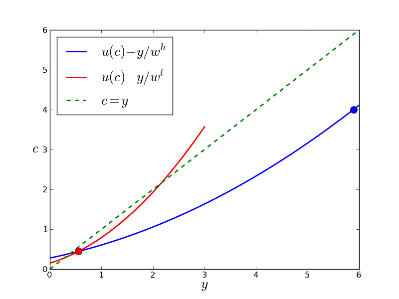
Optimal contracts for l-type and h-type
- l-type works less and consumes less than h-type
- h-type is indifferent between l and h contracts
- if we would redistribute a bit more to l-type, h-type would mimic
- both h-type and l-type pay taxes (contracts lie below the green line)
- h-type pays (a lot) more tax than l-type
- note that l-type does not want to mimic h-type: (\ref{eq:3}) is satisfied –which we needed to check
- tax function \(T(y)\) should be such that: \(c(y) = y - T(y)\) lies everywhere below the two indifference curves \(c^l = y^l - T(y^l)\) \(c^h = y^h - T(y^h)\)
- clearly there are a lot of functions \(T(y)\) that satisfy these criteria
- around \(y =6\) black line seems to be paralel to green line: coincidence?
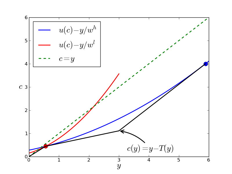
Example of tax function \(T(y)\) for implementation
What have we learned?
- Writing down an optimal taxation problem directly with a tax function \(T(y)\) is problematic
- Analytically, it is more convenient to write down the options for each type directly and make sure that each type chooses “his own” option by imposing IC constraints
- With optimal taxation we find that:
- high productivity type pays high tax (high average tax rate)
- but this does not imply that high type faces a (high) positive marginal tax rate
- in fact, marginal tax rate for high type equals 0
- no distortion at the top
- low type faces a positive marginal tax rate
- because high type wants to mimic low type, government needs to distort labor supply of low type (to make mimicking less attractive)
- labor supply is reduced with a positive marginal tax rate
- as high type works a lot, low type does not want to mimic high type
Monopolist (continuum of types)
Differences with optimal taxation
- Instead of considering two types, we now consider a continuum of types
- As people could not immigrate in the tax example, we only considered IC constraints
- when buying from a monopolist, one can decide not to buy at all: we need IR constraints
Model
- Monopolist can sell indivisible good to one consumer
- Cost of production equals 0 for monopolist
- If consumer buys the good from monopolist at price \(p\), his utility equals \(u(\theta) = \theta -p\) where \(\theta\) is distributed on \([0,1]\) with density [distribution] function \(f(\theta)[F(\theta)]\)
- Below we focus on a uniform distribution: \(f(\theta)=1,F(\theta) = \theta\)
- Monopolist cannot observe \(\theta\): this is private information for the consumer
- Revelation principle: monopolist asks consumer for his type \(\theta\)
- Given the consumer’s message \(\hat \theta\), he has to pay \(t(\hat \theta)\) and receives the good with probability \(x(\hat \theta)\)
- Consumer and monopolist are risk neutral: it does not matter whether the price is always paid (\(t\)) or only conditional on actually giving the good to the consumer (\(p=t/x\))
- Monopolist needs to choose \(x(.),t(.)\) in such a way that
- IC: consumer is willing to truthfully reveal \(\theta\)
- IR: consumer is willing to participate
- Monopolist maximizes expected revenue
Consumer’s optimization problem
- Consumer chooses message \(\hat \theta\) to solve
- Instead of looking at the first order condition for this problem, we use the envelope theorem:
- Since \(x(.)\) denotes a probability, we find that \(u'(\theta) \geq 0\)
- Hence the IR constraint \(u(\theta) \geq 0\) for all \(\theta \in [0,1]\) can be replaced by
as there is no reason for the monopolist to “give away presents”
- Consequently, we can write
Monopolist’s optimization problem
- Since \(t(\theta) = x(\theta)\theta - u(\theta)\), we can write the monopolist’s optimization problem as
- Using partial integration, we can write this as
- By increasing \(x(\theta)\), social surplus increases by \(\theta f(\theta)\)
- However, increasing \(x(\theta)\) makes it more attractive for types \(\theta'>\theta\) to mimic \(\theta\)
- To stop them from doing that, the monopolist needs to give them an informational rent: there are \(1-F(\theta)\) of these types above \(\theta\)
- This term is called marginal revenue (for reasons that become clear shortly)
- As the monopolist’s problem is linear in \(x(.)\), the solution is quite simple:
- With a uniform distribution we have \(MR(\theta) = 2\theta -1\)
- Hence the monopolist only sells to types with \(\theta \geq \frac{1}{2}\)
- Why does the monopolist not sell to everyone with valuation \(\theta\) above production costs 0?
Marginal Revenue
- To see where the term MR comes from in this context, we write \(q(\theta) = 1-\theta\)
- In a standard demand context, the people with a high value of the good are on the left hand side, while above they are on the right hand side of the interval \([0,1]\)
- Hence we “inverse things” with \(1-\theta\)
- Also if you set a price \(p\), how many people would buy?
- Consumers with \(\theta \geq p\) would buy and there are \(q = 1-p\) of such consumers
- The demand curve (consumer valuation) can now be written as \(1-q(\theta)\)
- Finally, \(MR(\theta) = [1-(1-\theta)] - \frac{1-\theta}{1} = 1 - 2q(\theta)\)
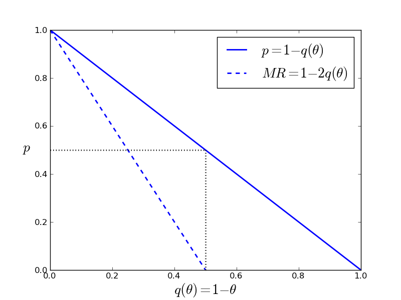
Demand curve and marginal revenue
Global optimum for consumer?
- The envelop theorem is a local argument, is it clear that the optimum supposed to be chosen (\(\hat \theta = \theta\)) by the consumer is a global optimum?
- What does the consumer optimization problem actually look like?
- To see this, first note that
- Hence, we see that
- Clearly, people with \(\theta < 0.5\) will not participate: they do not buy (\(x(\theta)=0\)) and they do not pay (\(t(\theta)=0\))
- For people with \(\theta \geq 0.5\), we see that \(x(\theta) =1\) and \(t(\theta)=0.5\)
- Hence we can write the consumer’s maximization problem as
- Either the consumer buys at a price equal to 0.5 or he does not buy at all
- Consumer only needs to reveal whether \(\theta\) is above 0.5 (or not)
- Put differently, the monopolist offers a menu with two options for \((x,t)\): \(\{(0,0),(1,0.5)\}\) and consumer chooses the best option from these two
- Truthful revelation of type is indeed a global optimum
- More generally, the reason why we can move from local to global here is the fact that \(x(\theta)\) is non-decreasing in \(\theta\)
What have we learned?
- Mechanism design can also be applied when there is a continuum of types
- in fact, this is often easier than the two type case
- A monopolist who faces a consumer without knowing the consumer’s valuation for the good should do the following:
- make a take-it-or-leave-it offer to the consumer
- consumer then decides whether to accept or reject
- this leads to social inefficiency (deadweight loss)
- to reduce informational rents of high types, monopolist does not sell to consumers who value the good more than the cost of production
- only consumers with a marginal revenue above the production cost can buy the good
- if marginal revenue is non-decreasing in type, we do not need to worry about the second order condition of the consumer optimization problem
Conclusion
Who needs mechanism design?
- If you want to analyze what the optimal policy is by, say, the government; instead of just analyzing the effects a specific policy (say a change in a linear tax rate), you need mechanism design
- Why should taxes be linear (only)?
- If you want to analyze a general tax function \(T(y)\), and you use a “standard approach”, the worker’s optimization problem may not be well defined
- Hard to check whether the local optimum for the worker is a global optimum
- Mechanism design forces you to think carefully about:
- objective function for the planner
- ways in which agents can deviate (incentive compatibility)
- whether agents want to participate (individual rationality) and what their outside options are (may differ with type: easier to emigrate for high than low productivity type)
- Mechanism design shows things generally:
- high type (in the examples above) is always better off than low type, no matter what the mechanism is (i.e. this is also true for mechanisms that are not optimal)
- high type can always mimic low type and then he is still better off
- if you would focus on linear tax functions, you would not see that marginal tax rate for highest type should be zero
- Important lesson from mechanism design: think in terms of informational rents
- make mechanism as efficient as possible (the bigger the total pie, the more rents you can extract)
- but make sure you do not leave too much rents to high types (who can mimic low types)