Lectures Methods: Python programming for economists
Table of Contents
- Introduction
- Lecture 1: The Power of Compounded Interest and Employment Dynamics
- Lecture 2: Healthcare expenditure
- App: Healthcare expenditure
- Python Code Explanation
- 1. Reading the data
- 2. Plotting the data
- 3. Defining a linear trend function
- 4. Fitting and visualizing the trend
- 5. Using optimization to find the best fit
- 6. Visualizing the optimal fit
- 7. Extending the model
- 8. Extrapolating the OLS Linear Trend to 2050
- 9. Multi-variable Regression: Adding GDP and OOP
- 10. Using a Numerical Solver (
fsolve) to Find Required OOP Levels - Summary of what the code does
- Review questions
- Lecture 3: Modeling Iteration
- Lecture 4: Search and Matching in the Labor Market
- App
- Python Code Explanation
- 1. Import libraries
- 2. Load the data
- 3. Model parameters from the literature
- 4. Matching function and wage equation
- 5. Estimating model parameters
- 6. Run the estimation
- 7. Compare model predictions to data
- 8. Interactive immigration shock (marimo slider)
- 9. Compute short‑run effects
- 10. Plot the wage curve
- Review questions
- Lecture 5: Modeling Dynamics
- Bibliography
Introduction
The idea of these lectures is to combine Python programing with economics. The overall goal is for you to acquire the skills to transfer information/knowledge to others (say, future colleagues) using more instruments than just written text.
Hence, we teach you how to use Python (learn the syntax) to solve economic models and then to create interactive apps to explain the intuition of these models. To explain how you can use these skills, we present all Python concepts in an economic context and show you how interactive elements can help the reader/user to gain the underlying economic intuition.
We start simple in lecture 1 with compound interest. Later you will learn how to solve for the equilibrium of models and do simulations. At the end you can solve differential equations.
The structure of each lecture is the same:
- explain the economic context
- show the intuition using an interactive notebook/app
- explain the python code that creates the app
- have some review questions
Our advice is to have this website open to read the information and next to it have your marimo notebook to make notes and program the interactive elements for the app. Most apps below are programed with streamlit which is very similar to marimo.
Lecture 1: The Power of Compounded Interest and Employment Dynamics
In this lecture we program two simple apps. First, we model compounded interest and then we model employment dynamics in a labor market. Along the way you learn the following Python concepts:
- variables
- lists and how to append lists
- for-loop
numpyandnumpyarrays, generating random numbers (e.g. from a binomial distribution)matplotlibto create figures- parameter sweep
Apps
This lecture introduces Python through two economic models:
- The Power of Compounded Interest: We model the growth of a bank account with regular deposits and compounded interest. This is analogous to the “falling coin” example in physics, but here we use an economic scenario.
- Modeling Employment and Unemployment: We model the employment status of 20 people in a village. Each person can be either employed or unemployed. At each time step, an employed person can lose their job (become unemployed) with a certain probability, and an unemployed person can find a job (become employed) with another probability.
You can experiment with both models in the interactive demos below.
Compounded interest
The following app illustrates how a lower monthly deposit can be “compensated” by a higher interest rate and lead to a higher final balance then a high monthly deposit with lower interest rate. Adjust the sliders by setting a relatively high deposit and low interest rate in scenario 1 and low deposit with high interest rate in scenario 2. Click the ’Calculate’ button to see how the balance develops over time in each scenario.
If the app does not load, open it in a new tab .
Employment dynamics
The following app illustrates how employment/unemployment evolves in a small town with 20 inhabitants. We start with full employment. With the sliders you can set the probability that an employee is fired (say, because her firm goes bankrupt) and the probability that an unemployed person is hired. Select the number of periods for which you want to run the simulation and click the ’Run Simulation’ button.
The second app illustrates a parameter sweep. This shows how sensitive an outcome is to the parameter value. In this case, we want to analyze the sensitivity of the long run unemployment level to the probability of finding a job. As this is a simple simulation model, we can actually derive the long run unemployment level analytically. The figure compares the simulated long run unemployment level with the analytic solution. For the probability of being fired chosen in the first app, clicking ’Sweep Parameter’ shows long run unemployment for different values of \(p_{hired}\).
If the app does not load, open it in a new tab .
Python Code Explanation
In this section we explain the Python code for the model itself, not yet for the interactive elements. In a next lecture we explain how to create sliders for parameters.
Compounded Interest Model
Let’s see how you can model the growth of a bank account with regular deposits and compounded interest in Python.
If you want to learn to program in Python, our advice is that you type the code below in your marimo notebook and run it. Then start to “play with it”: change things, experiment with the code. You cannot break anything and (mis)typing code, getting errors, using google or an LLM to understand the errors and change the code: this is how you learn to program. Just glancing over the code below and thinking you “understand things” is a waste of your time.
- 1. Set the parameters
We start by defining the monthly deposit, the monthly interest rate, and the number of months. Here, we use euros as the currency.
We do this by defining variables, like
deposit, and give these a value:deposit = 500 # euros per month rate = 0.003 # monthly interest rate (0.3%) months = 20 * 12 # 20 years - 2. Initialize the balance and create an empty list
We start with a balance of zero. We also create an empty
listcalledbalancesto store the account balance at each month.In Python, a
listis a data structure that can hold an ordered collection of items. In Python a list is denoted by brackets[]. “Ordered” in the sense that the first element refers to the start balance, the second element to the balance one month after that etc. We use a list here so we can keep track of the balance after each month, which is useful for plotting the results later.balance = 0 balances = [] - 3. Simulate the account growth with a for loop
We use a
forloop to repeat the same calculation for each month. In each iteration, we first store the current balance in the list, then update the balance by adding the deposit and applying the interest.for m in range(months + 1):This loop runs once for each month, including month 0.balances.append(balance)This adds the current balance to the end of thebalanceslist.
for m in range(months + 1): balances.append(balance) balance = balance * (1 + rate) + deposit - 4. Plot the results
We use
matplotlibto visualize the growth of the account over time.- for the code cell below we need to import two libraries
matplotlib,numpythat we use in the code. Staments likeimport numpy as npmean that we can accessnumpyfunctions likearangeby writingnp.arange - the
np.arangefunction takes three arguments: begin point, end point and step size; the end point is not included. In yourmarimonotebook: try different arguments in this function and see what the outcome is. years = np.arange(months + 1) / 12This creates a list of time points in years, matching the number of balances.plt.plot(years, balances)Theplotfunction takes two lists or arrays of equal length: the first for the x-axis, years, and the second for the y-axis, balances in euros.- By looking at the figure, you can probably infer what the functions
plt.xlabel, plt.ylabel, plt.titledo.
import matplotlib.pyplot as plt
import numpy as np

years = np.arange(months + 1) / 12
plt.plot(years, balances)
plt.xlabel("Years")
plt.ylabel("Account Balance (€)")
plt.title("Compounded Interest Over Time");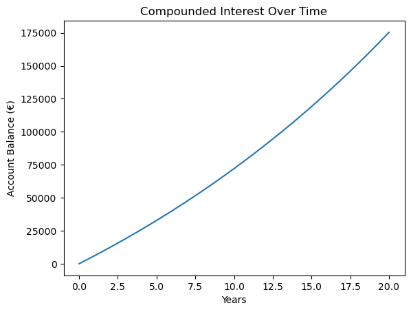
Use an LLM to figure out what the following Python code does:
periods = months + 1
factors = np.power(1 + rate, np.arange(periods))
balances = deposit * np.cumsum(factors)
- for the code cell below we need to import two libraries
Employment Dynamics Model
Let’s break down the Python code for simulating employment and unemployment in a small village.
- 1. Set the parameters
We define the number of people, the probabilities, and the number of time steps. Copy this into your
marimonotebook and see what happens if you change the value of the variablen_peopleto, say, 1000.n_people = 20 p_fired = 0.05 # probability an employed person is fired each step p_hired = 0.10 # probability an unemployed person finds a job each step n_steps = 100 - 2. Initialize the state
We start with everyone employed. We create lists to store the number of employed and unemployed people at each time step.
employed = n_people unemployed = 0 employed_hist = [employed] unemployed_hist = [unemployed] - 3. Simulate the process with a for loop
For each time step:
- For each employed person, we draw from a Bernoulli distribution to see whether they are fired. A Bernoulli distribution is equivalent to a binomial distribution with \(n=1\).
- For each unemployed person, we draw from a Bernoulli distribution to see whether they are hired.
- We update the counts and store them in the lists.
We use
np.random.binomial(n, p)to draw the number of successes, fired or hired, out ofnpeople, each with probabilityp.employed = employed - fired + hiredmeans that the new value ofemployed(left hand side) equals the previous value of this variable minus the people that are fired plus the hires this period.Above we have already seen the use of
appendto “add” a value to a list or an array.for t in range(n_steps): fired = np.random.binomial(employed, p_fired) hired = np.random.binomial(unemployed, p_hired) employed = employed - fired + hired unemployed = n_people - employed employed_hist.append(employed) unemployed_hist.append(unemployed) - 4. Plot the results
We use
matplotlibto plot the number of employed and unemployed people over time.When you add a label to a
plt.plotorplt.scattercommand withlabel="Employed", you need to specifyplt.legend()to add the legend to the figure. With the latter function you can also determine where the legend will be added in the figure. Google or use an LLM to find out how that works. If you do not specify a position,matplotlibwill try to find the best placement itself.steps = np.arange(n_steps + 1) plt.plot(steps, employed_hist, label="Employed") plt.plot(steps, unemployed_hist, label="Unemployed") plt.xlabel("Time step") plt.ylabel("Number of people") plt.title("Employment and Unemployment Over Time") plt.legend() plt.grid(True)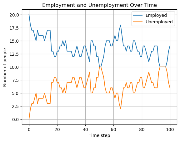
- Summary of what the code does
- Step 1: Set the parameters for the simulation.
- Step 2: Initialize the state and lists to store the results.
- Step 3: Use a for loop to simulate each time step, updating the state using random draws from the binomial distribution.
- Step 4: Plot the results to visualize how employment and unemployment evolve over time.
This model demonstrates how randomness and probabilities can be used to simulate real-world economic processes in
Python.
- Summary of what the code does
Parameter Sweep: Long-run Unemployment Rate
A question when doing simulations is: how sensitive are the simulation results to the parameter values chosen. One way to get an idea of this sensitivity is to run the simulations for a sweep of parameter values. We illustrate this by analyzing long run or steady state unemployment. In the simulations we program long run unemployment as follows:
- we run the simulations for 200 periods; this ensures that the effect of the initial unemployment level disappears
- then we consider only the final 50 periods (that is period 150-200)
- and we take the average unemployment level over these 50 periods; because hiring and firing are stochastic processes, the outcome in one particular period is random. By taking the average over 50 periods, we average out these per period stochastic outcomes.
As the model is quite simple, we can actually derive the steady state unemployment level analytically. If you do not quite see how we got this expression, you can watch the following derivation:
- 5. Sweep code
Two points on the code:
- here we use
np.linspaceinstead ofnp.arange. Both functions achieve the same result with slightly different syntax. Google “numpy linspace” for details. - in a later lecture we will look into indexing of lists and arrays. For now:
unemployment_hist[-50:]refers to the final 50 entries in list/arrayunemployment_hist.
n_people = 20 n_steps = 200 p_fired = 0.05 # fixed probability of being fired sweep_p_hired = np.linspace(0.1, 0.9, 30) avg_unemp = [] analytic_unemp = [] for p_h in sweep_p_hired: employed = n_people unemployed = 0 unemployed_hist = [unemployed] for t in range(n_steps): fired = np.random.binomial(employed, p_fired) hired = np.random.binomial(unemployed, p_h) employed = employed - fired + hired unemployed = n_people - employed unemployed_hist.append(unemployed) # Average unemployment rate over last 50 steps avg_unemp.append(np.mean(unemployed_hist[-50:]) / n_people) # Analytic steady-state u_analytic = p_fired / (p_fired + p_h) analytic_unemp.append(u_analytic) - here we use
- 6. Plotting the sweep results
plt.plot(sweep_p_hired, avg_unemp, label="Simulated (last 50 steps)")
plt.plot(sweep_p_hired, analytic_unemp, '--', label="Analytic steady-state")
plt.xlabel("Probability of finding a job")
plt.ylabel("Unemployment rate")
plt.title("Long-run Unemployment Rate vs. Probability of Finding a Job")
plt.legend()
plt.grid(True)
plt.show()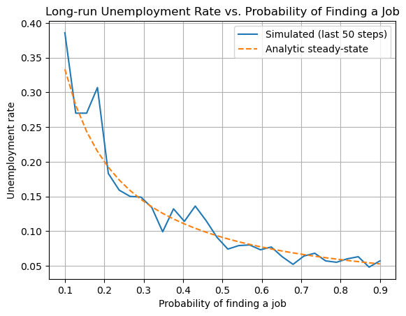
- Summary of what the code does
- Step 1-4: Simulate the employment dynamics as before.
- Step 5: For a range of probabilities of finding a job, run the simulation and compute the average unemployment rate in the long run. Also compute the analytic steady-state unemployment rate:
\[ u = \frac{p_{\text{fired}}}{p_{\text{fired}} + p_{\text{hired}}} \]
- Step 6: Plot both the simulated and analytic results to compare.
Sweeping parameters is a powerful way to explore how a model behaves as you change its assumptions.
- Summary of what the code does
Review Questions
Test your understanding of the Python concepts and models from this lecture. Each question gives you some code and context. For each:
- Explain what the code does (think before you look at the hint).
- Complete the code in your own notebook.
Question 1: Predicting the Future Value
You want to predict the future value of a savings account after 10 years, but you only know the monthly deposit and the interest rate. You are given the following code fragment:
deposit = 100
rate = 0.004
months = 10 * 12
balance = 0
for m in range(months):
    # update balance here
- a. Without running the code, explain how the balance will grow over time.
- b. Write code to print the balance every year (not every month).
- c. How would you modify the code to allow for a one-time bonus deposit in month 24?
For this question you need to use an if statement. Google “if statements in python” or get help from an LLM to solve this.
Hint / Solution
- The balance grows faster and faster due to compounding: each month, interest is earned on the previous balance.
- To print the balance every year, use an
ifstatement inside the loop:if m % 12 == 0: print(m//12, balance) - To add a bonus in month 24:
if m == 24: balance += bonus
Question 2: Unemployment Fluctuations
Suppose you want to simulate unemployment in a village, but you want to track the longest streak of consecutive months where unemployment is above 5 people.
n_people = 20
employed = n_people
unemployed = 0
p_fired = 0.05
p_hired = 0.10
longest_streak = 0
current_streak = 0
for month in range(months):
    # update employed and unemployed here
    if unemployed > 5:
        # update streaks here
- a. Explain how you would update
employedandunemployedeach month. - b. Complete the code to track the longest streak of high unemployment.
Hint / Solution
- Use random draws as before to update employment status.
- For streaks:
- If
unemployed > 5, incrementcurrent_streak. - If not, reset
current_streakto 0. - If
current_streak > longest_streak, updatelongest_streak.
- If
Question 3: Parameter Sweep Analysis
You want to analyze how the average unemployment rate (not steady state unemployment) changes as you sweep the probability of being fired.
Suppose you run a simulation for each value and store the results in a list called avg_unemp.
- a. How would you plot the results so that the x-axis shows the probability of being fired and the y-axis shows the average unemployment rate?
- b. Suppose the analytic solution does not match the simulation for very high or very low probabilities. List two possible reasons why.
Hint / Solution
- Use
plt.plot(p_fired_values, avg_unemp)wherep_fired_valuesis the list of probabilities you swept. - Possible reasons for mismatch:
- The simulation is too short to reach steady state for extreme probabilities.
- Random fluctuations are large in small populations, so the analytic solution (which assumes infinite population) is less accurate.
Lecture 2: Healthcare expenditure
App: Healthcare expenditure
If the app does not load, open it in a new tab .
Python Code Explanation
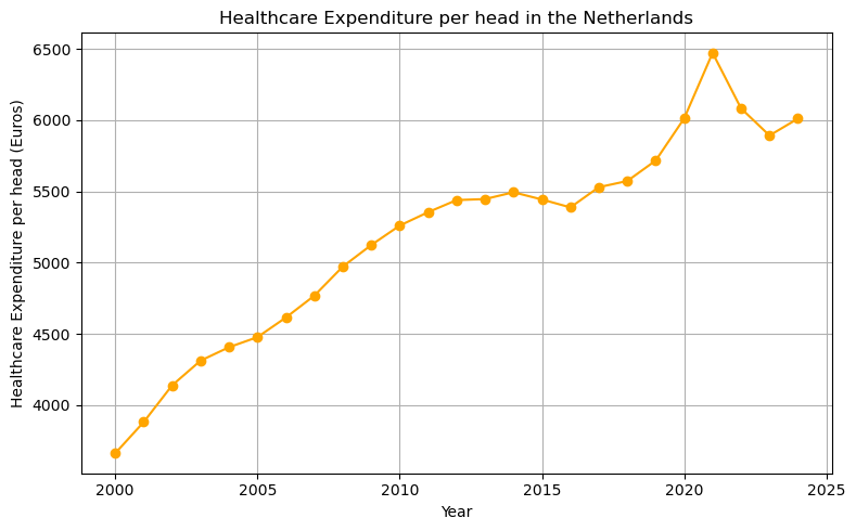
1. Reading the data
We use pandas to read the csv file with healthcare expenditure data for the Netherlands over the years 2000-2024. Here we just use the pd.read_csv= function, but with pandas you can also manipulate, clean data and merge dataframes. In the function call we specify the path where the csv file can be found: './data/gdp_healthcare_nl.csv'.
import pandas as pd

df = pd.read_csv('./data/gdp_healthcare_nl.csv')
df.head()
| Year | GDP_per_head | CHE_per_head | oop | |
|---|---|---|---|---|
| 0 | 2000 | 48561.827540 | 3660.652613 | 11.031692 |
| 1 | 2001 | 50301.690772 | 3879.911114 | 10.466823 |
| 2 | 2002 | 53515.311837 | 4137.932375 | 9.812201 |
| 3 | 2003 | 55703.272834 | 4311.324170 | 9.605323 |
| 4 | 2004 | 55797.445718 | 4405.689931 | 9.960184 |
The columns/variables in this dataframe df are the year of observation, GDP per head, healthcare expenditure per head and the percentage of healthcare expenditure that people pay out-of-pocket (oop).
2. Plotting the data
We use matplotlib to plot healthcare expenditure per head over time. Use google or an LLM to find out what plt.grid, plt.tight_layout do.
import matplotlib.pyplot as plt

plt.figure(figsize=(8,5))
plt.plot(df.Year, df.CHE_per_head, marker='o', color='orange')
plt.xlabel('Year')
plt.ylabel('Healthcare Expenditure per head (Euros)')
plt.title('Healthcare Expenditure per head in the Netherlands')
plt.grid(True)
plt.tight_layout()
3. Defining a linear trend function
Now we define our first function in Python. A function is a reusable block of code. Here, we define a function to compute a linear trend. We start with the keyword def specify the name of the function (which you are free to choose yourself but there are some restrictions on the name you choose) and then between parentheses ’()’ you specify the arguments of the function. That is, the variables that the function needs to calculate its results.
Here, the function has three arguments: years, intercept and slope. The function returns intercept + slope * (years - years.iloc[0]). Although this is not clear from the function definition, intercept and slope will be scalars and years is a vector (actually a pandas series). The syntax iloc[0] chooses the first element of this series. With df.Year as loaded from our data above, df.Year.iloc[0] equals 2000. The intercept equals linear_trend in the year 2000 and the trend slope applies to years \(> 2000\).
def linear_trend(years, intercept, slope):
    return intercept + slope * (years - years.iloc[0])
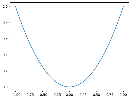
If you want to practice with defining (simpler) functions, do something like the following in your marimo notebook. Note that x**2 is Python syntax for \(x^2\).
def f(x):
    return x**2

range_x = np.linspace(-1,1,50)
plt.plot(range_x,f(range_x));
4. Fitting and visualizing the trend
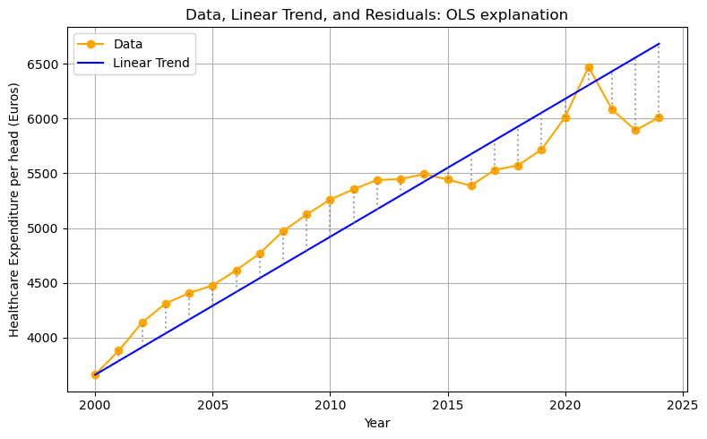
We plot the data, the linear trend, and the residuals (shown as vertical differences). Since the variable years is a vector, the function linear_trend returns a vector as well (a value for each year in years).
The Python syntax zip(years,che,trend) creates the combinations of the variables years,che,trend. After running the code block below in your marimo notebook (to make sure the variables are defined) you can evaluate for x, y, yhat in zip(years, che, trend): print(x, y, yhat) to see what zip does.
Finally, there is a new matplotlib command: plt.vlines: you give it three arguments: the \(x\) coordinate, the low value for \(y\) and high value for \(y\) between which a vertical line is drawn. linestyle=':' creates a dotted line.
years = df.Year
che = df.CHE_per_head
intercept = 3660.0
slope = 126.0
trend = linear_trend(years, intercept, slope)

plt.figure(figsize=(8,5))
plt.plot(years, che, marker='o', label='Data', color='orange')
plt.plot(years, trend, label='Linear Trend', color='blue')
for x, y, yhat in zip(years, che, trend):
    plt.vlines(x, min(y, yhat), max(y, yhat), color='gray', linestyle=':', alpha=0.7)
plt.xlabel('Year')
plt.ylabel('Healthcare Expenditure per head (Euros)')
plt.title('Data, Linear Trend, and Residuals: OLS explanation')
plt.legend()
plt.grid(True)
plt.tight_layout()
5. Using optimization to find the best fit
Above we just chose some values for intercept and slope. Now we will try to find the values that give the best fit. We follow OLS in defining “best” as minimizing the sum of squared residuals.
We use scipy.optimize.minimize to find the intercept and slope that minimize the sum of squared residuals. We define the function rss which has as arguments the parameters (intercept and slope), the years (independent variable) and healthcare expenditure che as dependent variable. By specifying y = che (or years=years) in the function definition of rss we give the function default values: if we do not specify y (or years) in our function call, Python will work with the specified default values for these variable.
Within the function definition of rss we call the function linear_trend that we defined above. The function np.sum sums the vector in its argument. To see how this works, run the code np.sum(np.arange(4)) in your marimo notebook.
The function minimize from scipy expects (at least) two arguments: the function that needs to be minimized (rss in this case) and an initial guess for the parameters, x0. We specify our initial guess as intercept = slope = 0 via x0 = [0,0].
The outcome of the minimization routine is captured in the variable res. After running the following code block in your notebook, you can evaluate res. This variable res has the Python type dictionary and one of the keys is x: the x value where the function rss is minimized. It contains the optimal intercept and optimal slope.
from scipy.optimize import minimize
import numpy as np

def rss(params, years=years, y=che):
    intercept, slope = params
    yhat = linear_trend(years, intercept, slope)
    return np.sum((y - yhat) ** 2)

res = minimize(rss, x0=[0, 0])
opt_intercept, opt_slope = res.x
print(res.x)
[4038.28659643 95.0425062 ]
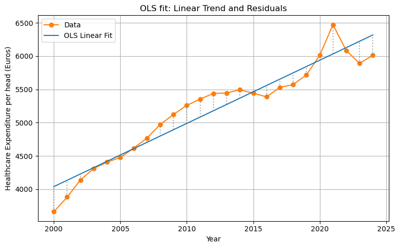
6. Visualizing the optimal fit
Now we can plot our data with the time trend that gives the best fit. To find the OLS regression line, we call our function linear_trend with the years variable and the optimal values opt_intercept, opt_slope.
opt_trend = linear_trend(years, opt_intercept, opt_slope)

plt.figure(figsize=(8,5))
plt.plot(years, che, marker='o', label='Data', color='tab:orange')
plt.plot(years, opt_trend, label='OLS Linear Fit', color='tab:blue')
for x, y, yhat in zip(years, che, opt_trend):
    plt.vlines(x, min(y, yhat), max(y, yhat), color='gray', linestyle=':', alpha=0.7)
plt.xlabel('Year')
plt.ylabel('Healthcare Expenditure per head (Euros)')
plt.title('OLS fit: Linear Trend and Residuals')
plt.legend()
plt.grid(True)
plt.tight_layout()
plt.show()
7. Extending the model
The fit of the OLS estimation is not bad. But we only used time (years) as explanatory variable. As healthcare is most likely a normal good, one would expect citizens to spend more on healthcare if they have higher incomes. On the macro level we can capture this with GDP per capita. Next to income, price is usually a determinant of expenditure on a good. Because the Netherlands has health insurance, people do not pay the full price of healthcare. But the deductible (part of healthcare expenditure that a patient pays her/himself) tends to reduce expenditure. Here we capture demand-side cost-sharing with the percentage that patients pay out-of-pocket (oop) for healthcare.
Below we will add these variables to our OLS regression to improve the fit.
8. Extrapolating the OLS Linear Trend to 2050
We can use the optimal OLS parameters to extrapolate the linear trend far into the future, for example to the year 2050. With the current information/data that we have, how much do we expect Dutch citizens to spend on healthcare (per capita) in 2050?
In order to predict (extrapolate) healthcare expenditure in 2050, we use our OLS regression line and substitute years till 2050 in the regression.
We define a new variable future_years starting from the first year (selecting using [] and index 0) and up till (but not including) 2051. Python starts counting at 0 and when specifying a range with range or np.arange the end point is not included.
Because we used the method iloc in our definition of linear_trend, we need to transform future_years into a pandas series.
future_years = np.arange(df.Year[0], 2051)
future_years_df = pd.Series(future_years)
future_trend = linear_trend(future_years_df, opt_intercept, opt_slope)

plt.figure(figsize=(10,5))
plt.plot(df.Year, df.CHE_per_head, marker='o', label='Observed Data', color='orange')
plt.plot(future_years, future_trend, label='OLS Linear Extrapolation (to 2050)', color='blue')
plt.xlabel('Year')
plt.ylabel('Healthcare Expenditure per head (Euros)')
plt.title('OLS Linear Extrapolation of Healthcare Expenditure per Head (to 2050)')
plt.legend()
plt.grid(True)
plt.tight_layout();
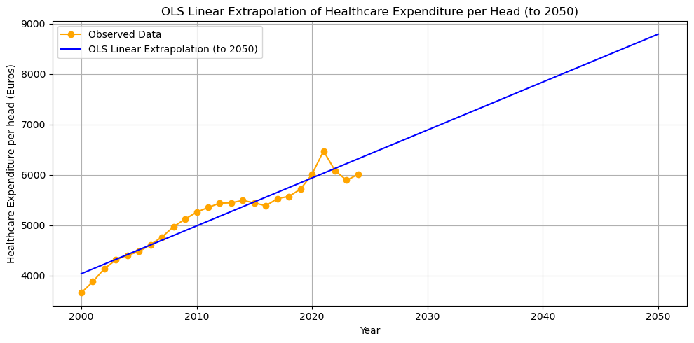
The model predicts that healthcare expenditure will be almost 9000 euros per capita in 2050. This is not necessarily a convincing prediction. First, it is not obvious that the trend should be linear. Perhaps the relation over time is concave (like \(\ln(x)\)) and grows more slowly than a linear function would suggest. If the relation is convex (like exponential growth) the situation will be (far) worse in 2050 in terms of public financing.
Second, the linear trend predicts healthcare expenditure growth that (most likely) exceeds GDP growth. This cannot be sustained by an economy and the government is likely to adopt measures to slowdown the growth in healthcare expenditure. One option is to increase demand-side cost-sharing. As people have to pay more out-of-pocket for healthcare treatments, they will tend to consume less.
9. Multi-variable Regression: Adding GDP and OOP
We can improve the fit of the model by including additional covariates: GDP per head and the percentage of healthcare expenditure paid out-of-pocket (oop).
def rss_multi(params, years=df.Year, gdp=df.GDP_per_head, oop=df.oop, y=df.CHE_per_head):
    intercept, slope_year, slope_gdp, slope_oop = params
    year_base = years - years.iloc[0]
    yhat = intercept + slope_year * year_base + slope_gdp * gdp + slope_oop * oop
    return np.sum((y - yhat) ** 2)

init_params = [0, 0, 0, 0]
res_multi = minimize(
    rss_multi,
    x0=init_params
)
opt_intercept_m, opt_slope_year, opt_slope_gdp, opt_slope_oop = res_multi.x

year_base = df.Year - df.Year.iloc[0]
che_hat_multi = (
    opt_intercept_m
    + opt_slope_year * year_base
    + opt_slope_gdp * df.GDP_per_head
    + opt_slope_oop * df.oop
)

plt.figure(figsize=(10,5))
plt.plot(df.Year, df.CHE_per_head, marker='o', label='Observed Data', color='orange')
plt.plot(df.Year, che_hat_multi, marker='s', label='Multi-variable Prediction', color='green')
plt.plot(df.Year, opt_trend, marker='x', label='OLS Linear Fit', color='blue', linestyle='--')
plt.xlabel('Year')
plt.ylabel('Healthcare Expenditure per head (Euros)')
plt.title('Observed vs Multi-variable Model Prediction')
plt.legend()
plt.grid(True)
plt.tight_layout();
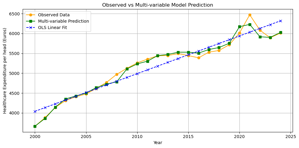
The fit is indeed better than the simple OLS linear trend.
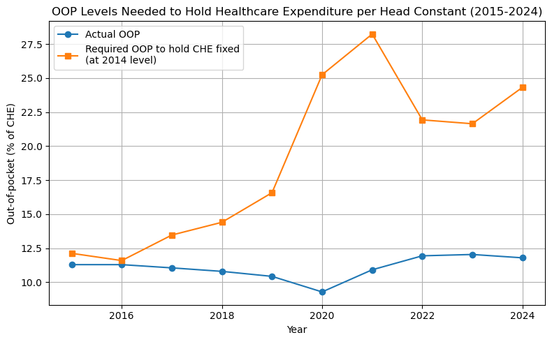
10. Using a Numerical Solver (fsolve) to Find Required OOP Levels
Suppose the government wants to keep healthcare expenditure constant. How can we find, for each year 2015–2024, the level of oop needed to keep healthcare expenditure per head at the 2014 level.
We use scipy.optimize.fsolve to solve for oop numerically.
First, we define the years years_proj over which we need to derive oop to keep expenditure constant at the 2014 level che_2014. Then we select gdp_proj for these years. In pandas you can make a selection with the [] notation, e.g. df[df.Year==2014]. When testing whether a variables is equal to a value we use ’='; in Python '’ is used for variables assignment (x=5 sets the variable x equal to 5). When there is a range of values, we use the .isin method: select all years in the range years_proj.
As above, we choose the base year as the first year in our series (that is how we estimated our OLS regression).
We define a function oop_to_hold_che which returns the difference between our prediction of healthcare expenditure yhat and the expenditure level in 2014. We will try to find the oop level that sets this function equal to zero: the predicted expenditure equals the 2014 expenditure. oop_to_hold_che has two arguments: the oop level that we try to find and the year y for which we want to find the oop level.
Finally, the function fsolve needs as inputs: the function oop_to_hold_che that we want to set equal to zero and an initial guess for the solution. The function oop_to_hold_che has two arguments: oop and the year y that we are considering. We are not trying to choose y to set the function equal to zero. Hence, we need to tell Python explicitly that it should think of oop_to_hold_che as a function of oop only (for each year y).
One way to do this would be to have different function names for oop_to_hold_che for each year, like oop_to_hold_che_2017. But this would be tedious. A better way is to use Python’s “anonymous” functions. These are functions without a name. You can define an anonymous function using the lambda keyword. As a silly example you can evaluate (lambda x: x + 5)(8) to get an idea what a lambda function does.
We set oop_to_hold_che equal to zero for the years 2015-2024 and add these values of oop to the list oop_needed. Then we plot this list together with the observed values of oop in our data.
from scipy.optimize import fsolve

che_2014 = df[df.Year == 2014]['CHE_per_head']
years_proj = np.arange(2015, 2025)
gdp_proj = df[df.Year.isin(years_proj)]['GDP_per_head'].values
year_base_proj = years_proj - df.Year.iloc[0]

def oop_to_hold_che(oop_guess,y):
    yhat = (
        opt_intercept_m
        + opt_slope_year * year_base_proj[y]
        + opt_slope_gdp * gdp_proj[y]
        + opt_slope_oop * oop_guess
    )
    return yhat - che_2014

oop_needed = []
for y in range(len(years_proj)):
    oop_init = df.oop[0]
    required_oop = fsolve(lambda x: oop_to_hold_che(x,y), oop_init)
    oop_needed.append(required_oop[0])

oop_data = df[df.Year.isin(years_proj)]['oop'].values

plt.figure(figsize=(8,5))
plt.plot(years_proj, oop_data, marker='o', label='Actual OOP')
plt.plot(years_proj, oop_needed, marker='s', label='Required OOP to hold CHE fixed\n(at 2014 level)')
plt.xlabel('Year')
plt.ylabel('Out-of-pocket (% of CHE)')
plt.title('OOP Levels Needed to Hold Healthcare Expenditure per Head Constant (2015-2024)')
plt.legend()
plt.grid(True)
plt.tight_layout();
Summary of what the code does
- Reading the data: Load the healthcare expenditure, GDP per head, and out-of-pocket (oop) data into a
pandasdataframe. - Plotting the data: Visualize healthcare expenditure per head over time using
matplotlib. - Defining a linear trend function: Create a Python function that computes a linear trend given years, intercept, and slope.
- Fitting and visualizing the trend: Plot the data, an example linear trend, and show residuals (vertical differences between data and trend).
- Using optimization to find the best fit: Use
scipy.optimize.minimizeto find the intercept and slope that minimize the sum of squared residuals (OLS fit). - Visualizing the optimal fit: Plot the data and the resulting OLS regression line with residuals.
- Extending the model: Discuss that only using time is limited and that other variables like income (GDP per head) and patient payments (oop) may matter.
- Extrapolating the OLS Linear Trend to 2050: Use the OLS results to predict future healthcare expenditure up to 2050 and plot the (possibly unrealistic) extrapolation.
- Multi-variable Regression: Improve the fit by adding GDP per head and oop as covariates in a multi-variable regression, and compare the fitted values to the data and simple trend.
- Using a Numerical Solver (
fsolve): For each future year, usefsolveto determine the oop needed to keep expenditure constant at 2014 levels, plot the required vs. actual oop, and discuss the relevance for policy.
Review questions
Question 1: Create Your Own Multi-variable Regression
Fit a new regression model that predicts healthcare expenditure per head using only GDP per head (not year or oop). Plot the predicted values versus the actual data. How does the fit compare to the simple linear trend?
Hint / Solution
Define a function like:
def rss_gdp(params, gdp=df.GDP_per_head, y=df.CHE_per_head): intercept, slope_gdp = params yhat = intercept + slope_gdp * gdp return np.sum((y - yhat) ** 2)- Use
minimize()to find the optimal coefficients. - Plot observed data and predicted values from this GDP-only model.
- Compare visually to the linear time trend fit.
—
Question 2: Use fsolve to Find the GDP Needed to Keep Expenditure Constant
Suppose you want to know, for a certain year (e.g., 2024), what value of GDP per head would keep healthcare expenditure fixed at its 2014 level, holding all else constant. Write a function and use fsolve to solve for this GDP value using your multi-variable model.
Hint / Solution
- Use your multi-variable coefficients from the previous regression (e.g., with GDP, OOP and year).
- For the selected year, plug in all other variables (year and oop) as they are in the data; solve for the value of GDP that sets the model prediction equal to the 2014 expenditure level.
Your function for
fsolveshould look like:def gdp_to_hold_che(gdp_guess): yhat = intercept + slope_year * (year - base_year) + slope_gdp * gdp_guess + slope_oop * oop return yhat - che_2014- Try different initial guesses and run
fsolve(gdp_to_hold_che, gdp_init).
Question 3: analyze the following three functions
For each of the following functions, do the following:
- plot the function on \(x \in [-10,10]\),
- find the zeros of the function (that is, the values of \(x\) where \(f(x)=0\)),
- find the extrema (minimum, maximum) of the functions.
The functions are: \(f(x) = x^3 - 3x + 1\), \(g(x) = \sin(2x)\) and \(h(x) = x^2 - 6 \sin(x)\).
Use google or an LLM to find the relevant Python functions for this. Python has only functions to minimize, how do you maximize a function? Most routines require you to specify a starting point of the algorithm. How does the starting point affect the outcome?
Lecture 3: Modeling Iteration
In this lecture you will learn:
- how to make interactive apps with Python in
marimo, - how to define sliders for parameters values and then use these parameters values to make plots,
- to program with
if, elifandelseclauses - use
forloops to model iteration, e.g. to solve a model over time - define a system of difference equations and work with it through matrix notation.
Apps
In terms of economics, we consider three models:
- an adverse selection model and how the market can unravel with asymmetric information,
- a duopoly Cournot model and how best-response iterations lead to the Nash equilibrium,
- a dynamic labor market model with three states: unemployed, low wage jobs, high wage jobs.
Adverse selection dynamics
The following app models an adverse selection market. Well known examples of such markets are the second-hand car markets (with “lemons”) and (health) insurance markets. In each of these markets there is asymmetric information. The seller of the car has used the car herself. She knows how (aggressively) she has driven the car, taken care of the car, investments in car maintenance etc. For the buyer this is not so clear. In the health insurance market, the insurer offers contracts to insure healthcare costs. The consumer has more information on his own health than the insurer does. Does he have a (chronic) disease? Does he have a healthy diet, exercise regularly etc.
The equilibrium in these markets tend to be inefficient: there is less trade than would be optimal from a welfare point of view. With the next app you can see how this inefficiency is affected by parameter values.
One interpretation of the iteration in the app is that agents react to what they saw in the previous period. In a health insurance context this would be: an insurer sells a health insurance contract, some consumers buy the contract and the price of the contract in the next period is the average costs of the contract in this period. If this price is rather high, some healthy people will decide not to buy health insurance because it is too expensive. This increases the average cost of the contract for the insurer (conditional on buying the contract, the customers have lower health and higher healthcare expenditure). So in period 3 the insurance premium increases again, perhaps inducing some of the healthier customers to forego insurance etc.
This process is called the unraveling of the market or a death spiral.
The context of the app is more like the second-hand car market: sellers value their car at \(q\) and are willing to sell to any buyer who pays a price above \(q\). Each car is worth more to the buyer than to the seller but the buyer cannot observe \(q\). If people are only willing to sell their car if \(q
If the app does not load,
open it in a new tab
.
Cournot best response dynamics
This app considers a Cournot market with two firms producing a homogenous good at constant marginal cost \(c\). Demand is of the form \(p = p(q_1+q_2)\). Hence, firm \(i\) maximizes profits
\begin{equation} \pi_i = \max_q p(q+q_j)q - c q \end{equation}with \(j \neq i \in \{1,2\}\) taking the output of the other firm as given.
Assume that demand is linear: \(p(q_1+q_2)=1-q_1-q_2\). Take the first order condition, say for firm 1, and show that this can be written as \(1-2q_1-q_2-c=0\) and derive the optimal reaction function \(r_1(q_1)\) shown in the app.
One way to derive the Nash equilibium is to use iterated best responses: start with an initial guess for \(q_1\) denoted by \(q_1^0\). Calculate firm 2’s optimal reaction: \(q_2^1=r_2(q_1^0)\). Then find 1’s optimal reaction to this: \(q_1^2 = r_1(q_2^1)\) etc. The figure shows you this process. In this case, these iterations converge to the Nash equilibrium.
If the app does not load, open it in a new tab .
Unemployment dynamics
Suppose we have an inelastic labor supply normalized to a mass of 1. Labor can be in one of three states: unemployed, employed in a low wage job and employed in a high wage job.???continue here???
If the app does not load, open it in a new tab .
Click here if you need a matrix multiplication refresher
Matrix notation is nothing more than that: notation. However, it turns out to be very powerful. You have (probably) seen matrices before. The following clips give a short refresher.
First we give a simple example of matrix multiplication with numbers so you can check the calculations easily.
Using the same visuals as the clip above we show the equivalence of the transition equations in the app above.
Python Code Explanation
Adverse Selection Model
In the adverse selection model, sellers have goods of quality \(q\) uniformly distributed on \([v_0, v_1]\). Sellers only offer goods if the market price \(p \geq q\). Buyers value quality at a mark-up:
\[ p = \mathrm{markup} \times E(q \mid q < p) \]
The equilibrium is found by iterating this price update until convergence.
Python code in Marimo:
import marimo as mo
import numpy as np
import matplotlib.pyplot as plt

v0 = mo.ui.slider(0, 100, value=50, label="Lowest quality $v_0$")
v1 = mo.ui.slider(1, 200, value=100, label="Highest quality $v_1$")
markup = mo.ui.slider(1.01, 2.0, value=1.2, step=0.01, label="Consumer mark-up")

mo.hstack([v0,v1,markup])
def expected_q_given_p_uniform(p, a, b):
    if p < a:
        return None
    elif p >= b:
        return (a + b) / 2
    else:
        return (a + p) / 2

def update_price_uniform(p, a, b, markup):
    expected_q = expected_q_given_p_uniform(p, a, b)
    if expected_q is None:
        return 0
    return markup * expected_q

p = markup.value * v1.value
history = []
for _ in range(50):
    history.append(p)
    new_p = update_price_uniform(p, v0.value, v1.value, markup.value)
    if abs(new_p - p) < 1e-6:
        break
    p = new_p
plt.plot(history)
The code above uses Marimo sliders for the parameters. The function expected_q_given_p_uniform computes the expected quality conditional on \(q < p\). The price update is iterated until convergence.
Cournot Duopoly Model
In the Cournot model, two firms choose quantities \(q_1\) and \(q_2\). The market price is
\[ p = 1 - q_1 - q_2 \]
and each firm has marginal cost \(c\). The best response functions are:
\[ q_1 = \frac{1 - q_2 - c}{2}, \qquad q_2 = \frac{1 - q_1 - c}{2} \]
The Nash equilibrium is found by iteratively updating each firm’s quantity.
Python code in Marimo:
import marimo as mo
import numpy as np
import matplotlib.pyplot as plt

c = mo.ui.slider(0, 0.99, value=0.2, step=0.01, label="Marginal cost $c$")
q1_init = mo.ui.slider(0, 0.99, value=0.45, step=0.01, label="Initial $q_1$")
n_iter = mo.ui.slider(2, 30, value=14, step=1, label="Number of iterations")
mo.hstack([c,q1_init,n_iter])
def reaction1(q2, c):
    return (1 - q2 - c) / 2

def reaction2(q1, c):
    return (1 - q1 - c) / 2

q1 = q1_init.value
points = []
for i in range(n_iter.value):
    if i % 2 == 0:
        q2 = reaction2(q1, c.value)
        points.append((q1, q2))
    else:
        q1 = reaction1(q2, c.value)
        points.append((q1, q2))
plt.plot(np.array(points)[:,0],np.array(points)[:,1])
plt.scatter(*points[0],label="initial $q_1$")
plt.legend()
plt.xlabel('$q_1$')
plt.ylabel('$q_2$')
The code above shows how the Cournot best responses are iterated, starting from an initial \(q_1\).
From scipy.optimize use the root function to calculate the Cournot equilibrium. You can use an LLM to help you with this.
Hint
- Define a function like:
def fixed_point(x,c):
    q1, q2 = x
    return  [
        # q1 minus firm 1's optimal response,
        # q2 minus firm 2's optimal response
    ]
The call scipy.optimize.root with the function and a starting point for the algorithm.
Labour Market Markov Model
The labor market model has three states: unemployed (\(u\)), low wage (\(l\)), and high wage (\(h\)). The transitions are:
- \(\mu\): probability an unemployed worker finds a low wage job
- \(\lambda\): probability a low wage worker becomes high wage
- \(\delta_l\): probability a low wage worker loses their job
- \(\delta_h\): probability a high wage worker loses their job
The difference equations are:
\begin{align*} u_{t+1} &= u_t + \delta_l l_t + \delta_h h_t - \mu u_t \\ l_{t+1} &= l_t + \mu u_t - \lambda l_t - \delta_l l_t \\ h_{t+1} &= h_t + \lambda l_t - \delta_h h_t \end{align*}Python code in Marimo:
import marimo as mo
import numpy as np
import matplotlib.pyplot as plt

mu = mo.ui.slider(0.01, 0.5, value=0.1, step=0.01, label="Job finding rate $\mu$")
lambda_ = mo.ui.slider(0.01, 0.5, value=0.15, step=0.01, label="Learning rate $\lambda$")
delta_l = mo.ui.slider(0.01, 0.5, value=0.05, step=0.01, label="Low wage sep. $\delta_l$")
delta_h = mo.ui.slider(0.01, 0.5, value=0.02, step=0.01, label="High wage sep. $\delta_h$")
u0 = mo.ui.slider(0.0, 1.0, value=1.0, step=0.01, label="Initial unemployment $u_0$")

mo.hstack([mu,lambda_,delta_l,delta_h,u0])
T = 60
u_hist, l_hist, h_hist = [], [], []
u, l, h = u0.value, 1 - u0.value, 0.0

for t in range(T):
    u_hist.append(u)
    l_hist.append(l)
    h_hist.append(h)
    new_l = mu.value * u
    l_to_h = lambda_.value * l
    l_to_u = delta_l.value * l
    h_to_u = delta_h.value * h

    next_u = u + l_to_u + h_to_u - new_l
    next_l = l + new_l - l_to_h - l_to_u
    next_h = h + l_to_h - h_to_u

    total = next_u + next_l + next_h
    next_u, next_l, next_h = next_u / total, next_l / total, next_h / total

    u, l, h = next_u, next_l, next_h

plt.plot(u_hist,label="unemployment")
plt.plot(l_hist,label="low wage employment")
plt.plot(h_hist,label="high wage employment")
plt.legend()
plt.xlabel("time")
plt.ylabel("fraction employed/unemployed")
This code simulates the labor market Markov process using Marimo sliders for all parameters.
We can also derive the labor market dynamics using matrix notation in Python. We can rewrite the above difference equations as follows:
\begin{equation} \begin{bmatrix} u_{t+1} \\ l_{t+1} \\ h_{t+1} \end{bmatrix} = \begin{bmatrix} 1 - \mu & \delta_l & \delta_h \\ \mu & 1 - \lambda - \delta_l & 0 \\ 0 & \lambda & 1 - \delta_h \end{bmatrix} \begin{bmatrix} u_t \\ l_t \\ h_t \end{bmatrix} \end{equation}- TODO
- use manim to explain matrix multiplication
We can define the transition matrix as follows:
A = np.array([
    [1-mu.value, delta_l.value, delta_h.value],
    [mu.value, 1-lambda_.value-delta_l.value,0],
    [0, lambda_.value,1-delta_h.value]
])
And then derive the employment dynamics in the following way. Although this may look less intuitive at the start, note how much shorter the code is when we use matrix notation. Matrix multiplication is done by the
np.dot()statement.S = np.array([u0.value, 1 - u0.value, 0.0]).reshape(3, 1) for _ in range(T): S = np.hstack((S,np.dot(A,S[:,-1].reshape(3,1)))) plt.plot(S[0],label="unemployment") plt.plot(S[1],label="low wage employment") plt.plot(S[2],label="high wage employment") plt.legend() plt.xlabel("time") plt.ylabel("fraction employed/unemployed")
Review questions
1. Adverse Selection: Does Increasing Mark-Up Always Restore Trade?
Consider the adverse selection model with \(v_0=30\) and \(v_1=90\). Write Marimo code to:
- Plot the equilibrium price and fraction traded as the mark-up varies from 1.01 to 2.0.
- Is there always trade (fraction traded > 0) for any mark-up \(>1\)?
Hint / Solution
import numpy as np
import matplotlib.pyplot as plt

v0, v1 = 30, 90
markups = np.linspace(1.01, 2.0, 100)
eq_prices = []
fractions = []

def expected_q_given_p_uniform(p, a, b):
    if p < a:
        return None
    elif p >= b:
        return (a + b) / 2
    else:
        return (a + p) / 2

for m in markups:
    p = m*v1  # start at high price
    for _ in range(30):
        expected_q = expected_q_given_p_uniform(p, v0, v1)
        if expected_q is None:
            break
        new_p = m * expected_q
        if abs(new_p - p) < 1e-6:
            break
        p = new_p
    eq_prices.append(p)
    frac = max(0, min(1, (p-v0)/(v1-v0)))
    fractions.append(frac)

plt.plot(markups, eq_prices, label="Equilibrium price")
plt.plot(markups, fractions, label="Fraction traded")
plt.xlabel("Markup")
plt.legend()
—
2. Cournot Duopoly: Add a Third Firm
Modify the Cournot duopoly Python code so there are three firms, each with marginal cost \(c\), facing demand of the form \(p = 1 - q_1 - q_2 - q_3\).
- Define best-response functions for each firm.
- Write a for loop to iterate best responses starting with initial quantities \(q_1=0.3, q_2=0.3, q_3=0.3\).
- Write a function
fixed_pointand use this function to solve for the equilibrium.
Hint / Solution
# Reaction for each: maximize (1 - sum(qs) - c)*q_i
def r1(q2, q3, c): return (1 - q2 - q3 - c)/2
def r2(q1, q3, c): return (1 - q1 - q3 - c)/2
def r3(q1, q2, c): return (1 - q1 - q2 - c)/2
c = 0.2
qs = [0.3, 0.3, 0.3]
history = [qs.copy()]
for i in range(15):
    qs[0] = r1(qs[1], qs[2], c)
    history.append(qs.copy())
    qs[1] = r2(qs[0], qs[2], c)
    history.append(qs.copy())
    qs[2] = r3(qs[0], qs[1], c)
    history.append(qs.copy())
plt.plot([row[0] for row in history], label='$q_1$')
plt.plot([row[1] for row in history], label='$q_2$')
plt.plot([row[2] for row in history], label='$q_3$')
plt.legend()
plt.xlabel("Step")
—
3. Labor Market: Steady State Without Iteration
Derive and plot the steady-state unemployment \(u^*\) as a function of the job-finding rate \(\mu\) (other parameters fixed at \(\lambda=0.1\), \(\delta_l=0.05\), \(\delta_h=0.03\)).
- Use the fact that in steady state, all variables don’t change over time.
Hint / Solution
Use google or an LLM to figure out what ’broyden1’ means. Why do we use x[0] below and not just x?
import numpy as np
from scipy import optimize
import matplotlib.pyplot as plt

lambda_, delta_l, delta_h = 0.1, 0.05, 0.03
mus = np.linspace(0.01, 0.5, 100)
def matrix_A(mu):
 return np.array([
    [1-mu, delta_l, delta_h],
    [mu, 1-lambda_-delta_l,0],
    [0, lambda_,1-delta_h]
    ])

def fixed_point(x,mu):
    x = (x/np.sum(x)).reshape(3,1)
    return x - np.dot(matrix_A(mu),x)

u_star = []
for mu in mus:
    x = optimize.root(lambda x: fixed_point(x,mu), [1/3.0, 1/3.0, 1/3.0], method='broyden1', tol=1e-14).x
    u_star.append(x[0])
plt.plot(mus,u_star)
plt.xlabel(r'$\mu$ (job finding rate)')
plt.ylabel('Steady state $u^*$')
—
4. Matrix Notation: Simulation With Numpy Only
In the labor market model, implement the time path simulation using only Numpy arrays and matrix multiplication (not manually updating variables).
- Set up the transition matrix for \(\mu=0.12\), \(\lambda=0.09\), \(\delta_l=0.04\), \(\delta_h=0.03\), \(u_0=0.8\).
- Plot the evolution of all three states.
Hint / Solution
mu, lmbd, dl, dh = 0.12, 0.09, 0.04, 0.03
A = np.array([
    [1 - mu, dl, dh],
    [mu, 1 - lmbd - dl, 0],
    [0, lmbd, 1 - dh]
])
S = np.array([0.8, 0.2, 0]).reshape(3,1)
history = [S.flatten()]
for _ in range(60):
    S = np.dot(A, S)
    S = S / np.sum(S)   # (optional: renormalize so they sum to 1)
    history.append(S.flatten())
history = np.array(history)
plt.plot(history[:,0], label="Unemployed")
plt.plot(history[:,1], label="Low wage")
plt.plot(history[:,2], label="High wage")
plt.legend()
plt.show()
—
5. Extending the Labor Model: Add a Direct High Wage Offer Channel
Suppose a fraction \(\alpha\) of unemployed directly get a high wage job each period. The equations become:
\begin{align*} u_{t+1} &= u_t + \delta_l l_t + \delta_h h_t - \mu u_t - \alpha u_t \\ l_{t+1} &= l_t + \mu u_t - \lambda l_t - \delta_l l_t \\ h_{t+1} &= h_t + \lambda l_t + \alpha u_t - \delta_h h_t \end{align*}- Write Marimo code to simulate the process, using sliders for \(\mu, \lambda, \delta_l, \delta_h, u_0, \alpha\).
- Plot over time.
- What happens as \(\alpha\) increases?
Hint / Solution
mu = mo.ui.slider(0.01, 0.5, value=0.1, label="Job finding rate")
lambda_ = mo.ui.slider(0.01, 0.5, value=0.15, label="Learning rate")
delta_l = mo.ui.slider(0.01, 0.5, value=0.05, label="Low wage sep.")
delta_h = mo.ui.slider(0.01, 0.5, value=0.02, label="High wage sep.")
alpha = mo.ui.slider(0.0, 0.2, value=0.0, step=0.01, label="Direct high wage $\alpha$")
u0 = mo.ui.slider(0.0, 1.0, value=1.0, step=0.01, label="Initial unemployment")
mo.hstack([mu,lambda_,delta_l,delta_h,alpha,u0])
T = 60
u_hist, l_hist, h_hist = [], [], []
u, l, h = u0.value, 1-u0.value, 0.0

for t in range(T):
    u_hist.append(u)
    l_hist.append(l)
    h_hist.append(h)
    to_l = mu.value * u
    to_h = alpha.value * u
    l_to_h = lambda_.value * l
    l_to_u = delta_l.value * l
    h_to_u = delta_h.value * h

    next_u = u + l_to_u + h_to_u - to_l - to_h
    next_l = l + to_l - l_to_h - l_to_u
    next_h = h + l_to_h + to_h - h_to_u

    total = next_u + next_l + next_h
    next_u, next_l, next_h = next_u/total, next_l/total, next_h/total

    u, l, h = next_u, next_l, next_h

plt.plot(u_hist,label="unemployment")
plt.plot(l_hist,label="low wage")
plt.plot(h_hist,label="high wage")
plt.legend()
As \(\alpha\) increases, the fraction in high wage employment rises and steady-state unemployment falls.
Lecture 4: Search and Matching in the Labor Market
In this lecture you will learn:
- How to translate an economic question into two sub-problems:
- what data can I use?
- what model is useful for this question?
- Use papers from the economics literature to calibrate parameters and use data to estimate (other) parameters.
- Define your own function to find the estimator that minimizes the sum of squared residuals.
- Use the model to simulate the outcomes of different scenarios.
App
Suppose after graduating you are hired by the Dutch Ministry of Social Affairs. In parliament there have been recurring discussions about immigration. The minister asks you to give her an idea of the potential effects of immigration on unemployment and wages in the Netherlands. Suppose immigration increases by 50%, or even doubles. What would happen to unemployment and wages?
To answer this question we need two ingredients: data and an economic model. Before reading on, it may be useful to think about how you would approach this question yourself. There are many ways to model the effects of immigration. Below we develop one example using data from Statistics Netherlands (CBS) and a search and matching framework. We then use this model to build a small simulation in Python.
The goal is not to obtain a precise prediction. Rather, we want to give the minister a sense of the order of magnitude of the effects. To build intuition, we construct an interactive model where immigration can increase by anywhere between 0% and 100%.
For this exercise we focus on immigration from outside Europe (EU and EFTA) with the motivation to work in the Netherlands.
A key advantage of the search and matching framework is that it focuses on flows in the labor market rather than the entire stock of workers. Workers search for jobs and firms post vacancies. Matches occur when searching workers and vacancies meet through the matching process.
Asylum migration can also affect the labor market, but these effects are more indirect and occur with a lag. For example, asylum procedures can take several years before individuals are allowed to participate in the labor market. For simplicity, we abstract from these effects here.
In the search framework, an increase in immigration initially increases the number of job seekers. However, the number of vacancies is not fixed in the long run. Firms respond to changes in labor market conditions by posting more vacancies. The interaction between workers and firms determines unemployment, vacancies, and wages.
The key elements of the framework are:
- Workers and firms meet via a matching function.
- Wages are determined by Nash bargaining.
- Immigration acts as an exogenous increase in labor supply.
- Firms respond to a larger labor supply by posting more vacancies.
Model structure
Notation:
- \(U\): number of unemployed workers
- \(V\): number of vacancies
- \(M\): number of matches between workers and firms
- \(\theta = V/U\): labor market tightness
The matching process is described by a Cobb–Douglas matching function:
\[ M = m U^\alpha V^{1-\alpha} \]
where \(m\) measures matching efficiency and \(\alpha\) is the elasticity of matches with respect to unemployment.
A useful quantity is the job-finding probability for unemployed workers:
\[ \frac{M}{U} = m \theta^{1-\alpha} \]
This expression shows that job finding increases when the labor market becomes tighter (more vacancies relative to unemployed workers).
Wage determination
Wages are determined through Nash bargaining between the worker and the firm. The wage splits the surplus of the match.
In our simplified framework, the outside option of the worker depends on how easily a job can be found. When the labor market is tight and jobs are easy to find, the value of remaining unemployed is higher.
We capture this idea in reduced form by specifying the worker’s outside option as
\[ b \theta^{1-\alpha} \]
where \(b\) summarizes factors such as welfare benefits and institutions that affect the value of unemployment.
Given Nash bargaining with worker bargaining power \(\beta\), the wage becomes
\[ w = b \theta^{1-\alpha} + \beta \left(a - b \theta^{1-\alpha}\right) \]
where
- \(w\): wage
- \(a\): worker productivity
- \(\beta\): worker bargaining power
This equation shows that wages increase with productivity and with labor market tightness.
From the literature (Mortensen and Nagypál 2007; Petrongolo and Pissarides 2001) we calibrate
\[ \alpha = 0.5, \quad \beta = 0.5 \]
The remaining parameters \(m\), \(a\), and \(b\) will be estimated using Dutch data.
Data
To estimate the model for the Netherlands we use data from CBS:
- unemployment https://www.cbs.nl/en-gb/figures/detail/80590eng
- vacancies https://www.cbs.nl/en-gb/figures/detail/84545ENG
- wages https://opendata.cbs.nl/#/CBS/en/dataset/85663ENG/table
The relevant variables are:
- \(U\): “Unemployed labour force / seasonally adjusted (x 1,000)”
- \(V\): “Vacancies seasonally adjusted, unfilled (x 1,000)”
- \(M\): “Vacancies seasonally adjusted, filled (x 1,000)”
The variable \(M\) represents the number of vacancies filled during a period and is therefore a proxy for the flow of matches.
The dataset is stored in: ./data/labour_data.csv
We estimate the parameters \(m\), \(a\), and \(b\) by minimizing the sum of squared differences between model predictions and the observed data for matches and wages.
Immigration shock
Our research question is: what happens when immigration increases?
From the CBS migration statistics we observe that roughly 14,000 people per year migrate to the Netherlands with the explicit intention of joining the labor market. Using the table
https://opendata.cbs.nl/#/CBS/nl/dataset/80016ned/table
with the following selections:
- men and women
- age \(\geq 15\)
- all countries of birth
- migration motive: joining the labour force
we obtain approximately 14,000 migrants per year in the early 2000s.
We interpret these migrants as entering the labor market as job seekers. In other words, they initially increase unemployment \(U\).
Short-run effect
In the short run we assume that the number of vacancies is fixed. Firms cannot immediately adjust their vacancy postings.
When immigration increases, the number of unemployed workers \(U\) rises while vacancies \(V\) remain fixed. As a result, labor market tightness
\[ \theta = V/U \]
falls.
Lower tightness reduces the job-finding probability and lowers the worker’s outside option. Through the Nash bargaining equation this leads to lower wages.
Long-run adjustment
In the longer run firms can respond by creating additional vacancies. Firms post vacancies until the expected profit from a vacancy equals the cost of posting it.
The expected benefit of posting a vacancy equals the probability of filling it times the profit generated by a match.
The probability that a vacancy is filled is
\[ q(\theta) = \frac{M}{V} = m \theta^{-\alpha} \]
The free-entry condition for vacancies is therefore
\[ c = q(\theta)(a - w) \]
where \(c\) is the cost of posting a vacancy.
This condition determines equilibrium labor market tightness in the long run.
After an immigration shock, firms gradually create additional vacancies until the free-entry condition holds again. As a result, labor market tightness and wages move back toward their original equilibrium levels, while the total number of vacancies increases.
Effect of immigration
The Streamlit app below allows you to explore these mechanisms. You can simulate increases in immigration between 0% and 100% and observe how unemployment, vacancies, labor market tightness, and wages respond in both the short run and the long run.
If the app does not load, open it in a new tab .
Python Code Explanation
1. Import libraries
We first import the Python packages used for data handling, estimation, and plotting.
import numpy as np
import pandas as pd
import matplotlib.pyplot as plt
from scipy.optimize import minimize, fsolve
import marimo as mo
—
2. Load the data
We load the CBS dataset containing unemployment, vacancies, matches, and a wage index.
df = pd.read_csv("./data/labour_data.csv")
df.head()
Important columns in the dataset:
Unemployed labour force/Seasonally adjusted (x 1,000)→ unemployment \(U\)Vacancies seasonally adjusted, unfilled (x 1000)→ vacancies \(V\)Vacancies seasonally adjusted, filled (x 1000)→ matches \(M\)Average_monthly_wage_index→ wage index
—
3. Model parameters from the literature
The search-and-matching literature suggests that we can calibrate \(\alpha\) and \(\beta\) at 0.5 (Mortensen and Nagypál 2007; Petrongolo and Pissarides 2001).
alpha = 0.5
beta = 0.5
These values imply:
- unemployment and vacancies contribute symmetrically to matching
- workers and firms split the surplus equally.
—
4. Matching function and wage equation
We now write a function that predicts matches and wages for a given observation.
def predict_row(row, m, a, b, counterfactual_immigration=0):

    U = row['Unemployed labour force/Seasonally adjusted (x 1,000)'] + counterfactual_immigration
    V = row['Vacancies seasonally adjusted, unfilled (x 1000)']

    # Matching function
    M_pred = m * (U**alpha) * (V**(1-alpha))

    # Labor market tightness
    theta = V / U

    # Wage equation (Nash bargaining)
    wage_pred = beta * a + (1 - beta) * b * (theta ** (1 - alpha))

    return M_pred, wage_pred
This function implements two key model equations:
- Matching: \(M = m U^α V^{1−α}\)
- Wage: \(w = βa + (1−β)b θ^{1−α}\)
—
5. Estimating model parameters
We estimate the unknown parameters:
- matching efficiency \(m\)
- productivity \(a\)
- outside option parameter \(b\)
We do this by minimizing the sum of squared errors between the model and the data.
def sum_squared_errors(params, df):

    m, a, b = params
    errors = []

    for _, row in df.iterrows():

        M_pred, wage_pred = predict_row(row, m, a, b)

        e_M = (row['Vacancies seasonally adjusted, filled (x 1000)'] - M_pred)**2
        e_wage = (row['Average_monthly_wage_index'] - wage_pred)**2

        errors.append(e_M + e_wage)

    return np.sum(errors)
This function computes how far the model predictions are from the data.
—
6. Run the estimation
We now use a numerical optimizer to estimate the parameters.
init_params = [0.8, 200, 50]

result = minimize(sum_squared_errors, init_params, args=(df,))

m_hat, a_hat, b_hat = result.x

m_hat, a_hat, b_hat
The optimizer searches for parameter values that make the model fit the observed data as closely as possible.
—
7. Compare model predictions to data
Using the estimated parameters, we compute predicted matches and wages.
M_pred = []
wage_pred = []

for _, row in df.iterrows():
    mp, wp = predict_row(row, m_hat, a_hat, b_hat)
    M_pred.append(mp)
    wage_pred.append(wp)
Now we plot observed vs predicted values.
periods = df['PeriodQ'].astype(str)
fig, axs = plt.subplots(1,2, figsize=(12,4))

axs[0].plot(periods, df['Vacancies seasonally adjusted, filled (x 1000)'])
axs[0].plot(periods, M_pred)
axs[0].set_title("Matches")
axs[0].set_xticks(periods[::4])
axs[0].tick_params(axis='x', rotation=45)


axs[1].plot(periods, df['Average_monthly_wage_index'])
axs[1].plot(periods, wage_pred)
axs[1].set_title("Wages")
axs[1].set_xticks(periods[::4])
axs[1].tick_params(axis='x', rotation=45)

plt.tight_layout()
fig
The purpose of this step is simply to check whether the model roughly reproduces the data.
—
8. Interactive immigration shock (marimo slider)
In the app, immigration is controlled with a slider.
In marimo we create the same interaction using a widget.
immigration_slider = mo.ui.slider(
    start=0,
    stop=100,
    step=1,
    value=0,
    label="Immigration increase (%)"
)
The slider allows the user to simulate immigration increases between 0% and 100%.
—
9. Compute short‑run effects
We use the latest observation as the baseline and simulate additional immigrants entering unemployment.
immigration_slider
latest = df.iloc[-1]

U0 = latest["Unemployed labour force/Seasonally adjusted (x 1,000)"] * 1000
V0 = latest["Vacancies seasonally adjusted, unfilled (x 1000)"] * 1000

immigrants_per_year = 14000

additional = immigrants_per_year * immigration_slider.value / 100

U = U0 + additional
theta = V0 / U

w = beta * a_hat + (1 - beta) * b_hat * theta**(1 - alpha)

theta, w
Short run assumption:
- immigration increases unemployment
- vacancies remain fixed
This reduces labor market tightness \(θ = V/U\) and lowers wages.
—
10. Plot the wage curve
Finally we visualize how immigration moves the economy along the wage curve.
theta0 = V0 / U0

theta_grid = np.linspace(0.5*theta0, 1.5*theta0, 200)

w_grid = beta * a_hat + (1 - beta) * b_hat * theta_grid**(1 - alpha)

fig, ax = plt.subplots()

ax.plot(theta_grid, w_grid)
ax.scatter(theta, w)

ax.set_xlabel("Labor market tightness θ")
ax.set_ylabel("Wage index")

plt.show()
Interpretation:
- the curve shows wages implied by Nash bargaining
- immigration increases unemployment
- this lowers tightness \(θ\)
- the economy moves left along the wage curve, reducing wages.
Review questions
Question 1. Simulating the matching function
Write a Python function that computes the number of matches \(M\) using the matching function
\(M = m U^\alpha V^{1-\alpha}\)
Choose parameter values \(m = 0.8\) and \(\alpha = 0.5\). Simulate how matches change when unemployment \(U\) increases from 50 to 200 while vacancies \(V = 100\) remain fixed. Plot matches as a function of unemployment.
Hint / Solution
import numpy as np
import matplotlib.pyplot as plt

m = 0.8
alpha = 0.5
V = 100

U = np.linspace(50, 200, 100)

M = m * (U**alpha) * (V**(1-alpha))

plt.plot(U, M)
plt.xlabel("Unemployment U")
plt.ylabel("Matches M")
plt.title("Matching Function")
plt.show()
Question 2. Job-finding probability
The probability that an unemployed worker finds a job is
\(p(\theta) = m \theta^{1-\alpha}\)
where \(\theta = V/U\).
Write Python code that computes and plots the job-finding probability for \(\theta\) values between 0.2 and 2.
Hint / Solution
import numpy as np
import matplotlib.pyplot as plt

m = 0.8
alpha = 0.5

theta = np.linspace(0.2, 2, 100)

p = m * theta**(1-alpha)

plt.plot(theta, p)
plt.xlabel("Labor market tightness θ")
plt.ylabel("Job-finding probability")
plt.title("Job-finding probability")
plt.show()
Question 3. Wage curve
The wage equation in the lecture is
\(w = \beta a + (1-\beta)b\theta^{1-\alpha}\)
Assume \(a = 200\), \(b = 50\), \(\alpha = 0.5\), \(\beta = 0.5\).
Write Python code that plots the wage curve for \(\theta\) between 0.2 and 2.
Hint / Solution
import numpy as np
import matplotlib.pyplot as plt

a = 200
b = 50
alpha = 0.5
beta = 0.5

theta = np.linspace(0.2, 2, 100)

w = beta * a + (1-beta) * b * theta**(1-alpha)

plt.plot(theta, w)
plt.xlabel("Labor market tightness θ")
plt.ylabel("Wage")
plt.title("Wage curve")
plt.show()
Question 4. Immigration shock in the short run
Suppose the labor market initially has
U = 200 (thousand unemployed) V = 150 (thousand vacancies)
Immigration increases unemployment by 20%.
Write Python code that
• computes the initial tightness \(θ_0\) • computes the new tightness after immigration • computes the corresponding wages using the wage equation.
Hint / Solution
import numpy as np

a = 200
b = 50
alpha = 0.5
beta = 0.5

U0 = 200
V = 150

theta0 = V / U0

U1 = U0 * 1.2
theta1 = V / U1

w0 = beta * a + (1-beta) * b * theta0**(1-alpha)
w1 = beta * a + (1-beta) * b * theta1**(1-alpha)

print(theta0, theta1)
print(w0, w1)
Question 5. Estimating the matching function
Using the matching function
\(M = m U^\alpha V^{1-\alpha}\)
generate simulated data for \(U\) and \(V\), compute \(M\), and then estimate the parameters \(m,\alpha\) using least squares.
Hint: rearrange the equation as
\(m = M / (U^\alpha V^{1-\alpha})\)
Compute the average value of \(m\) from your simulated observations.
Hint / Solution
import numpy as np

alpha = 0.5
m_true = 0.8

np.random.seed(0)

U = np.random.uniform(50, 200, 100)
V = np.random.uniform(50, 200, 100)

M = m_true * (U**alpha) * (V**(1-alpha)) + np.random.normal(0,10,100)
Now define a matching function as a function of \(m,\alpha\), derive the residuals between the matching function and the observed values for \(M\). Minimize the sum of squared residuals.
Lecture 5: Modeling Dynamics
In this lecture you will learn:
- How to solve differential equations using
scipy. - Understand the economic intuition for dynamic effects and illustrating this using interactive apps.
- Solve dynamic optimization problems.
Solving Dynamic Economic Models
Much of economics is about understanding how things change over time. Capital accumulates gradually, firms learn from experience, and contracts must account for incentives that evolve across different types of consumers. These processes are inherently dynamic: what happens today influences what happens tomorrow.
To study such problems formally, economists often describe economic forces with differential equations. These equations capture how key variables evolve as a function of their current level and economic incentives. In many cases the models cannot easily be solved analytically, but modern numerical tools allow us to compute their behavior and visualize the implied dynamics.
The following three apps introduce three economic environments in which dynamics play a central role. Each example highlights a different type of dynamic reasoning commonly used in economic research.
Apps
Solow model
One of the most fundamental questions in macroeconomics is why some countries are richer than others and how economies grow over time. A key mechanism behind long‑run growth is capital accumulation: societies invest part of their income in machines, infrastructure, and technology that increase future production.
However, capital does not grow automatically. Investment increases the capital stock, but depreciation and population growth work in the opposite direction. New workers require additional capital to maintain capital per worker and productivity, and existing capital gradually wears out.
The Solow growth model captures this tension between investment and dilution. In this framework, the economy produces output using capital and labor. A constant fraction of output is saved and invested, which increases the capital stock. At the same time, depreciation and population growth reduce the amount of capital available per worker.
These forces determine how capital per worker evolves over time. If the economy starts with very little capital, investment will exceed depreciation and capital will grow rapidly. If the economy becomes very capital‑intensive, depreciation and population growth eventually dominate, slowing further accumulation.
This dynamic adjustment leads to a steady state: a level of capital per worker at which investment exactly offsets depreciation and population growth. At this point the capital stock per worker stops changing.
An important question is how the steady state depends on economic parameters. For example, how would the long‑run level of capital change if households saved a larger fraction of their income? What happens if population growth increases? How does the productivity of capital affect the outcome?
Thinking through these questions helps build intuition for the forces that determine long‑run economic development.
If the app does not load, open it in a new tab .
Mechanism design
Many markets involve asymmetric information. Firms often do not know exactly how much each consumer values their product. Some customers are willing to pay a lot, while others are much more price sensitive.
Consider a monopolist selling a product whose quality or quantity can vary. Consumers differ in how much they value this quality, but the firm cannot observe their valuation directly. If the firm could perfectly observe each consumer’s type, it could tailor a price to each individual and extract all surplus. In reality, the firm must design a pricing strategy that induces consumers to reveal their preferences voluntarily.
This leads to the problem of mechanism design or screening. The firm offers a menu of contracts, where each contract specifies a quantity or quality level together with a price. Consumers choose the option that maximizes their own utility.
The difficulty is that high‑valuation consumers might pretend to be low‑valuation consumers if the low‑quality contract is cheaper. To prevent this, the menu must be designed so that each consumer prefers the option intended for their own type. This requirement is called incentive compatibility or truthful revelation.
Ensuring truthful behavior typically forces the firm to leave some surplus –often called information rents– to higher-valuation consumers. These rents are the price the firm must pay to obtain information about consumers’ willingness to pay.
The resulting optimal contracts display several interesting patterns. Higher types typically receive higher quality and pay higher prices. At the same time, the allocation is generally distorted relative to the socially efficient outcome, especially for low‑valuation consumers.
Understanding these distortions is central to many areas of economics, including regulation, taxation, insurance, and pricing strategies in digital markets.
Click here if you need a refresher on the envelope theorem
The envelope theorem is a property of optimization problems that economists tend to use a lot. The following clip explains what it is and illustrates the envelope theorem with a simple example.
Click here if you need a refresher on the Euler equation
The Euler equation is used in dynamic optimization problems.
We will use the Euler equation in two applications below. In these applications, we optimize over two variables and for one of these variables the objective function does not depend on the time derivative of this variable. Hence, we have a problem like:
\[ \max_{x,y} \int_{t_0}^{t_1} f(t,x(t),y(t),x'(t))dt \]
Then the Euler equation implies that the first order conditions are:
\[ \frac{\partial f}{\partial x} - \frac{d}{dt} \left( \frac{\partial f}{\partial x'} \right) = 0 \]
and for \(y(t)\):
\[ \frac{\partial f}{\partial y} = 0 \]
because \(\frac{\partial f}{\partial y'} = 0\).
If the app does not load, open it in a new tab .
Learning by doing
Firms often become more efficient as they gain experience with a production process. This phenomenon, known as learning by doing, has been documented in many industries such as semiconductor manufacturing, aircraft production, and renewable energy technologies.
When firms produce more today, they accumulate knowledge that reduces future production costs. This creates a dynamic trade-off. Producing more in the present may reduce current profits, but it can increase future profitability by lowering costs.
Because of this trade-off, firms may choose production paths that differ from the static profit-maximizing quantity. A purely static monopolist would simply choose the output level that maximizes current profits given current costs. A forward‑looking firm, however, takes into account that higher production today accelerates learning and reduces costs tomorrow.
This introduces an investment motive in production decisions. Output today not only generates current revenue but also contributes to the firm’s stock of experience.
Several interesting questions arise in this environment. Should firms produce more or less early in the life of a product? How does the importance of the future –captured by the discount rate– affect production choices? And how does the value of accumulated experience change over time?
Analyzing these questions helps illustrate how dynamic optimization differs from static decision making. When future benefits are important, firms may deliberately deviate from short‑run profit maximization in order to improve long‑run outcomes.
If the app does not load, open it in a new tab .
Python Code Explanation
Interactivity in Marimo
In marimo, interactive elements are created with mo.ui widgets.
Example:
import marimo as mo

alpha = mo.ui.slider(0.1, 0.9, value=0.3, step=0.01, label="Capital share (α)")
s = mo.ui.slider(0.01, 0.6, value=0.2, step=0.01, label="Savings rate")
Then display them:
alpha, s
To use the value inside calculations:
alpha.value
s.value
Marimo automatically re-runs dependent cells when a widget value changes.
So if a plot depends on alpha.value, it updates automatically when the alpha slider moves.
—
Solving Differential Equations in SciPy
Two numerical solvers are used in the apps.
- Initial Value Problems (IVP)
Used in App 1.
An IVP has the structure
y'(t) = f(t, y)
y(t0) = y0
Meaning:
- we know the starting value
- we simulate the path forward in time.
SciPy function:
scipy.integrate.solve_ivpBasic syntax:
solve_ivp(function, t_span, y0, t_eval=grid)Arguments:
function: defines the differential equationt_span: time interval(t0, T)y0: initial valuet_eval: grid of times where the solution is reported
The solver internally uses numerical integration methods (typically an algorithm called Runge–Kutta).
The result object contains:
sol.t     time grid
sol.y     solution values
—
- Boundary Value Problems (BVP)
Used in App 2 and App 3.
A BVP specifies conditions at different points, e.g.
y(a) = value1
y(b) = value2
Instead of simulating forward from a known starting value, the algorithm must search for a function that satisfies both boundaries simultaneously.
SciPy function:
scipy.integrate.solve_bvpBasic structure:
solve_bvp(system, boundary_conditions, x_grid, initial_guess)Inputs:
system(x,y)→ differential equationsboundary_conditions(ya,yb)→ conditions at start and endx_grid→ grid for solutioninitial_guess→ guess for the solution path
The solver iteratively adjusts the path until the differential equations and boundary conditions hold.
The result object includes
sol.x     grid
sol.y     solution
sol.yp    derivatives
—
Solow Growth Model
- Model equation
Capital evolves according to
k'(t) = s k^α − (n + δ) kThis is a single differential equation. And we have a given capital stock \(k(0)=k_0\) at the start of time: initial value problem.
—
- Step 1: Import libraries
import numpy as np
import matplotlib.pyplot as plt
from scipy.integrate import solve_ivp
Roles:
numpy→ numerical operationsmatplotlib→ plottingsolve_ivp→ differential equation solver
—
- Step 2: Define parameters (interactive)
In marimo:
alpha = mo.ui.slider(0.1,0.9,value=0.3)
s = mo.ui.slider(0.01,0.6,value=0.2)
n = mo.ui.slider(0.0,0.05,value=0.01)
delta = mo.ui.slider(0.0,0.1,value=0.05)
k0 = mo.ui.slider(0.01,5.0,value=0.5)
Use them in calculations as
alpha.value—
- Step 3: Define the differential equation
def solow(t,k):
    return s.value*k**alpha.value - (n.value+delta.value)*k
Important detail:
SciPy expects the function signature
f(t,y)even if the equation does not depend on
t.—
- Step 4: Compute steady state
The steady state solves
0 = s k^α − (n+δ)kwhich gives
k_ss = (s.value/(n.value+delta.value))**(1/(1-alpha.value))—
- Step 5: Time grid
t_span = (0,50)
t_eval = np.linspace(0,50,200)
This means we simulate the model from time 0 to 50 and evaluate at 200 points.
—
- Step 6: Solve the IVP
sol = solve_ivp(solow, t_span, [k0.value], t_eval=t_eval)Note:
[k0]must be a list because SciPy allows systems of equations.Solution:
sol.t
sol.y[0]
—
- Step 7: Plot transition dynamics
plt.plot(sol.t, sol.y[0])
plt.axhline(k_ss)
Interpretation:
- the path converges toward the steady state.
—
- Step 8: Solow diagram
Create a grid of capital levels:
k_grid = np.linspace(0.01,5,200)Compute
investment = s.value*k_grid**alpha.value
break_even = (n.value+delta.value)*k_grid
Plot both curves.
Their intersection is the steady state.
—
Mechanism Design Model
This problem involves two differential equations:
u'(θ) = (θ − λ/f(θ))/c
λ'(θ) = −f(θ)
Boundary conditions:
u(θ_min) = 0
λ(θ_max) = 0
So this is a boundary value problem.
—
- Step 1: Define density
def f(t):
    return 1/(b-a)*np.ones_like(t)
This corresponds to a uniform distribution.
np.ones_like(t)ensures the function works for vector inputs needed in thescipyfunctions below.—
- Step 2: Define system of ODEs
def design(t,y):
    return np.vstack([
        (t - y[1]/f(t))/c,
        -f(t)
    ])
Interpretation:
yis a vector:y[0] = u(θ) y[1] = λ(θ)np.vstackstacks derivatives into a matrix required bysolve_bvp.—
- Step 3: Boundary conditions
def bc(ya,yb):
    return np.array([ya[0], yb[1]])
where
ya = solution at θ_min
yb = solution at θ_max
So the function enforces
u(θ_min)=0 # because index [0] in ya refers to u(θ): y[0]
λ(θ_max)=0 # because index [1] in yb refers to λ(θ): y[1]
—
- Step 4: Initial grid
t_eval = np.linspace(a,b,100)—
- Step 5: Initial guess
np.zeros((2, t_eval.shape[0]))Explanation:
- 2 equations
- guess values along the grid
—
- Step 6: Solve BVP
sol = solve_bvp(design, bc, t_eval, guess)After solving:
sol.y[0] = u(θ)
sol.y[1] = λ(θ)
—
- Step 7: Recover quantities and prices
The optimal quantity:
x = sol.yp[0]Because
u'(θ) = x(θ)and
yp[0]refers to the derivative (“y prime”) of the first element inywhich is \(u\).Price is derived from
p = θx − uso
p = t_eval*x - sol.y[0]—
Dynamic Pricing with Learning
This model also forms a BVP, but with time as the state variable.
State variables:
Q(t)      cumulative production
λ(t)      shadow value
Differential equations:
Q'(t)
λ'(t)
Boundary conditions:
Q(0) = 0
λ(T) = 0
—
- Step 1: Define system
def learning(t,y):State variables stored as
y[0] = Q
y[1] = λ
Then return derivatives.
scipyexpects the result stacked:np.vstack((dQdt, dlambdadt))—
- Step 2: Boundary conditions
def bc(ya,yb):
    return np.array([ya[0], yb[1]])
Meaning
Q(0)=0
λ(T)=0
—
- Step 3: Solve BVP
sol = solve_bvp(learning, bc, t_eval, guess)Extract solution:
Q = sol.y[0]
λ = sol.y[1]
q = sol.yp[0]
Since
Q'(t) = q(t)—
- Step 4: Static benchmark
The static monopoly solution is
q_static = (1 - c/(1+Q)) / 2Plot both:
dynamic q(t)
static q(t)
—
Review questions
Solow model
Create the Solow model in a marimo notebook and analyze the following:
- add technological growth
- plot the growth in output \(f(k)\) over time. How is this figure affected by the initial capital stock \(k_0\) and the saving rate \(s\)?
Mechanism design
In your marimo notebook:
- change the distribution
f(θ) - compare the information rent in the optimal solution with the information rent in the first-best allocation.
Learning-by-doing
In your marimo notebook:
- vary time horizon
T - introduce capacity constraints
- in competition policy cases there is a suspicion that firms that price below marginal costs (\(p < c\)) are trying to remove their competitors from the market to enjoy monopoly profits in the future. Discuss this suspicion in the light of this model.