Python: collusion with Bertrand competition
In this notebook we consider collusion with Bertrand competition. However, we do not specify a demand function. We start from consumers’ utility and then derive demand from that.
With Bertrand competition it turns out that defining the best response numerically is a bit tricky…
from scipy import optimize,arange
from numpy import array
import matplotlib.pyplot as plt
%matplotlib inline
utility structure and demand
Assume that a consumer buys either one product or none at all. A consumer of type \(n\) values buying a product at price \(p\) at \(n-p\). Her outside option is normalized at 0. Hence, she only buys the good if \(n-p \geq 0\).
Total demand is then given by all consumers with \(n \geq p\).
def u(p,n): # utility for consumer who values good at n
    return n-p

consumer_types = arange(0.0,1.01,0.01) # 100 consumers with n varying between 0 and 1

def buy(p,n):
    if u(p,n) >= 0:
        buy = 1.0
    else:
        buy = 0.0
    return buy

def total_demand(p): # total demand equals the sum of demands of consumers n for all consumer_types
    demand_vector = [buy(p,n)/len(consumer_types) for n in consumer_types]
    return sum(demand_vector)
profits and reaction functions
We consider a duopoly with firms 1 and 2. Consumers buy from the cheapest firm or choose a firm randomly if both charge the same price. Firm \(i\) has constant marginal cost of production \(c_i\) and no fixed cost.
Let \(x(p)\) denote total demand at price \(p\). Then profits equal:
With this profit function, firm \(i\) chooses \(p_i\) optimally, given \(p_j\). Analytically, this implies for \(p_j \in \langle c_1, p_1^m \rangle\) setting \(p_i = p_j -\varepsilon\) for \(\varepsilon > 0\) small.
Why can’t we use this here?
Give the intuition for the reaction function specified below; why is it not optimal?
def profit(p1,p2,c1):
    if p1 > p2:
        profits = 0
    elif p1 == p2:
        profits = 0.5*total_demand(p1)*(p1-c1)
    else:
        profits = total_demand(p1)*(p1-c1)
    return profits

def reaction(p2,c1):
    if p2 > c1:
        reaction = c1+0.8*(p2-c1)
    else:
        reaction = c1
    return reaction
equilibrium
We define the Bertrand equilibrium as a fixed point to a mapping from \(p_1,p_2\) to the optimal response of firm 1 and 2 to these values of \(p_1,p_2\). This is done in the same way as in the Cournot file.
We specify symmetric firms \(c_1=c_2=0.0\) and give initial guess \(p_0\) for equilibrium prices.
def vector_reaction(p,param): # vector param = (c1,c2)
    return array(p)-array([reaction(p[1],param[0]),reaction(p[0],param[1])])

param = [0.0,0.0] # c1 = c2 =0
p0 = [0.5, 0.5] # initial guess: p1 = p2 = 0.5

ans = optimize.fsolve(vector_reaction, p0, args = (param))
print ans
[ 4.94065646e-324 4.94065646e-324]
The outcome is what we would expect: \(p_1 = p_2 = c_1 = c_2 = 0.0\). Bertrand competition with homogeneous goods and constant average costs leads to price equal marginal costs.
collusion
Now we are going to see whether firms can collude on a price \(p\). As with Cournot, we focus on the symmetric case where \(c_1 = c_2 =c\) and \(p_1 = p_2 =p\).
With Cournot we defined the deviation (from collusion) profit using the firm’s optimal response.
Why don’t we use this here?
Why is the optimal deviation profit correct?
def collusion_profits(p,c,delta): # we only do this for the symmetric case: c1 = c2 = c
    profits = profit(p,p,c)
    ans = optimize.fsolve(vector_reaction, p0, args = ([c,c]))
    if profits >= (1-delta)*2*profits+delta*profit(ans[0],ans[1],c):
        industry_profits = 2*profits
    else:
        industry_profits = 0
    return industry_profits
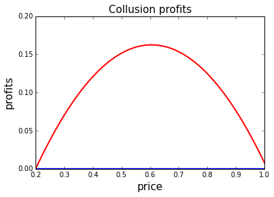
maximum collusion profits
To see which prices can be sustained as collusion profits and to see which price maximizes collusion profits, let’s plot collusion profits as a function of \(p\). Here we work with constant marginal costs equal to \(c = 0.2\).
The red line plots collusion profits for \(\delta_1 = 0.8\) and the blue line for \(\delta_2 = 0.4\).
Why is the blue line (if you can see it…) horizontal at 0?
What is the profit maximizing price with the red line?
How does this compare to the condition on collusion derived in the lecture?
c = 0.2
range_p = arange(0.0,1.01,0.01)
delta1 = 0.8
delta2 = 0.4

range_profits = [collusion_profits(p,c,delta1) for p in range_p]
range_profits_2 = [collusion_profits(p,c,delta2) for p in range_p]

plt.clf()
plt.plot(range_p, range_profits,'-', color = 'r', linewidth = 2)
plt.plot(range_p, range_profits_2,'-', color = 'b', linewidth = 2)
plt.title("Collusion profits",fontsize = 15)
plt.xlabel("price",fontsize = 15)
plt.ylabel("profits",fontsize = 15,rotation = 90)
plt.xlim(c,1.0)
plt.ylim(0.0,0.2)
plt.savefig('collusion_Bertrand.png')
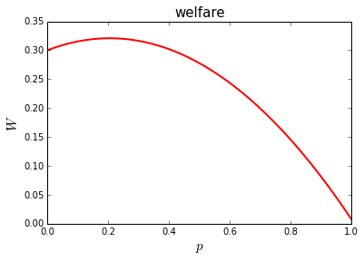
welfare
Finally, let’s consider total welfare as a function of price.
At which price \(p\) is welfare maximized? Why?
def welfare(p):
    welfare = sum([u(c,n)*buy(p,n)/len(consumer_types) for n in consumer_types])
    return welfare

range_welfare = [welfare(p) for p in range_p]

plt.clf()

plt.plot(range_p, range_welfare,'-', color = 'r', linewidth = 2)
plt.title("welfare",fontsize = 15)
plt.xlabel("$p$",fontsize = 15)
plt.ylabel("$W$",fontsize = 15)
plt.xlim(0.0,1.0)
plt.savefig('welfare.png')