Python: introduction
This notebook gives an introduction to the programming language python and the jupyter notebook.
When you are first reading this, you are probably looking at the html file. This file looks the same as the notebook, but you cannot run code in the html file (which you can in the notebook).
By reading the html file, you will learn:
how to install python
how to start the notebook
how to edit and typeset in the notebook
Starting the Notebook
The easiest way to start a new notebook is via the Anaconda Prompt in the Start Menu of Windows or via Terminal in iOS. From there you can Launch the Jupyter notebook –by typing ‘jupyter notebook’ and press ENTER– which will start the local server for Jupyter and open the explorer in your default browser.
By default you will see your local user directory. From here you can navigate into your documents or downloads folder, open a new notebook or create one. If you downloaded the notebooks into the downloads folder you can click on Downloads and then on the notebook you saved.
IMPORTANT Install Anaconda before the first session and go through this notebook before class to make sure it works for you!
Learning Python
Why would you want to learn Python? First of all, because it is fun! (well that is what we think…)
There are a number of ways to learn python:
http://quant-econ.net/py/learning_python.html gives a great introduction
Python for infomatics is a nice book; you can download it as ibook on your ipad/iphone and then it includes weblecturs
if you are interested, you can check out http://www.pyladies.com/about/
or just google on “python tutorial” and pick one that you like
Just to be sure: this is a course on Competition Policy and not on programming. There will be no Python questions on the exam.
But you can save yourself a lot of time on the assignments if you master the basics of Python. And you earn a point for class participation if you finish the datacamp course in time.
In the lectures we will give you Python examples that you can then copy-paste for your assignments. This saves you time when using python for the assignments. Also the assignments will be given in a notebook and some code may already be included.
Also when you finish your degree(s) and look for a job: Python is open source. Programs like Stata, Mathlab, Mathematica etc. are great, but they need a license (to be used legally). If your employer has no such license, you have a problem. Not with Python!
Markdown
A big advantage of the ipython notebook is that you can typeset equations to explain what you are doing. You type in a cell, but change the dropdown menu at the top of this page from “Code” to “Markdown”.
Again there are numerous introductions to markdown on the web. See, for instance, this on on the basics. Google “markdown tutorial” and choose your favourite one.
Although you may use MS Word to type documents and equations, this is actually not a very good choice for two reasons. First, as you will learn during the course, Microsoft is a bad company from a competition policy point of view. Hence, we cannot reward it by using its products. Second, the software is not great for our purposes.
To type equations in markdown, use latex. Double click on this cell in the notebook (i.e. not in the html version) to see how you create equations. Symbols can be put between dollar signs, like \(x\), \(\alpha\), \(y^2\) etc.
For an equation, type
There are lots of latex tutorials on the web, but mostly you can google what you want; like “latex phi” if you want to know how to type \(\phi\). But also “latex empty set”, “latex summation”, “latex integral” etc. Together with copying what I do, this will do for the assignments. There is no need to learn latex.
Doing your BA thesis in latex may force you to learn a lot in a short time, but you should definitely consider writing your MSc thesis in latex. For your BA thesis, writing it in markdown may actually be quite a good option. To move from markdown to pdf, I use pandoc which works brilliantly. Look here for some examples. Especially, the html slideshows with revealjs are great fun and so much better than powerpoint!
Some first code
We finish this file with typing some code. You can execute the code (and change it) in the notebook (but not in the html file).
This should give you some first ideas. In the lectures we will look at economic examples.
First, Python is a great calculator
1+1
2
Now something a bit bigger:
10**20
100000000000000000000
As you note, in Python \(10^{20}\) is written with ** not with ^.
We can define a variable \(x\)
x = 10
x+2
12
There are lists, tuples, dictionaries etc. Make sure you know what these different data types are and how they work.
We finish off with making a graph using matplotlib. Also look at the gallery if you want to know how to do things.
First, we need to import this library:
import matplotlib.pyplot as plt
%matplotlib inline
The first line says that we import matplotlib as “plt”. Hence statements referring to this start with “plt”, as you will see in a second. The second statement makes sure that we can see the graphs in the notebook as we make them.
Let’s define a function that we all know, so that we understand what we are drawing.
def my_first_function(x):
    return x**2
my_first_function(4)
16
Well, that works. Note that when you type “my_” you can press the “tab” key to get auto-completion. Saves a bit of time when typing; and you cannot accidently type the wrong name which leads to an error lateron.
Before we can plot this function, we define for which values of \(x\) we want to view this function. This is most easily done with the arange statement from scipy:
from scipy import arange

range_x = arange(-2.0,2.1,0.1)
print(range_x)
[ -2.00000000e+00  -1.90000000e+00  -1.80000000e+00  -1.70000000e+00
  -1.60000000e+00  -1.50000000e+00  -1.40000000e+00  -1.30000000e+00
  -1.20000000e+00  -1.10000000e+00  -1.00000000e+00  -9.00000000e-01
  -8.00000000e-01  -7.00000000e-01  -6.00000000e-01  -5.00000000e-01
  -4.00000000e-01  -3.00000000e-01  -2.00000000e-01  -1.00000000e-01
   1.77635684e-15   1.00000000e-01   2.00000000e-01   3.00000000e-01
   4.00000000e-01   5.00000000e-01   6.00000000e-01   7.00000000e-01
   8.00000000e-01   9.00000000e-01   1.00000000e+00   1.10000000e+00
   1.20000000e+00   1.30000000e+00   1.40000000e+00   1.50000000e+00
   1.60000000e+00   1.70000000e+00   1.80000000e+00   1.90000000e+00
   2.00000000e+00]
Hence, “arange” creates an array starting at \(-2.0\) going up to –but not including– \(2.1\) with steps \(0.1\). Note the scientific notation with \(e-01\). Finally, we are doing numerical stuff here, so \(0\) looks “a bit odd”.
Now we create a range of \(y\)-values that we want to draw. See how elegantly you define this new list of numbers:
range_y = [my_first_function(x) for x in range_x]
print(range_y)
[4.0, 3.6099999999999999, 3.2399999999999993, 2.8899999999999992, 2.5599999999999987, 2.2499999999999987, 1.9599999999999984, 1.6899999999999984, 1.4399999999999984, 1.2099999999999982, 0.99999999999999822, 0.80999999999999828, 0.63999999999999835, 0.48999999999999838, 0.35999999999999849, 0.24999999999999867, 0.15999999999999887, 0.089999999999999095, 0.039999999999999362, 0.0099999999999996619, 3.1554436208840472e-30, 0.010000000000000373, 0.040000000000000785, 0.090000000000001232, 0.1600000000000017, 0.25000000000000222, 0.36000000000000276, 0.49000000000000338, 0.64000000000000401, 0.81000000000000461, 1.0000000000000053, 1.210000000000006, 1.4400000000000068, 1.6900000000000077, 1.9600000000000084, 2.2500000000000093, 2.5600000000000103, 2.8900000000000112, 3.2400000000000122, 3.6100000000000132, 4.0000000000000142]
As we are working numerically here, some numbers look a bit strange. But when we plot it later on, it will look familiar again. If you want to look at one element in this list, type
range_y[0]
4.0
Note that Python starts counting at \(0\). That also means that:
range_y[41]
---------------------------------------------------------------------------

IndexError                                Traceback (most recent call last)

<ipython-input-11-366258d81fe1> in <module>()
----> 1 range_y[41]


IndexError: list index out of range
If you get an error like this, simply google “python list index out of range”: you are not the first to encounter this problem…
Lists have other properties that you may not expect. For instance, although they may look like vectors to you, they are not:
[5,6,7]-[1,1,1]
---------------------------------------------------------------------------

TypeError                                 Traceback (most recent call last)

<ipython-input-12-1683f32e17a9> in <module>()
----> 1 [5,6,7]-[1,1,1]


TypeError: unsupported operand type(s) for -: 'list' and 'list'
Hence you get an error. There are a number of solutions to this. Again google something like “python subtract lists” to see what other people have tried. Note that whereas I thought of \([5,6,7]-[1,1,1]\) as a vector operation, others see it as a set operation. What is the difference?
In order to work with lists as vectors, I tend to use
from numpy import array
print(array([5,6,7])-array([1,1,1]))
[4 5 6]
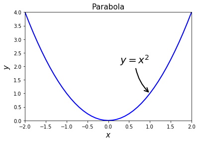
Back to our graph, here is how you plot and save it:
plt.clf() # starts a new graph
plt.plot(range_x, range_y,'-', color = 'b', linewidth = 2) # play around with colors like 'r', or styles like '--'
plt.title("Parabola",fontsize = 15)
plt.xlabel("$x$",fontsize = 15)
plt.ylabel("$y$",fontsize = 15)
plt.xlim(-2.0,2.0)
plt.ylim(0.0,4.0)
plt.annotate('$y=x^2$', xy=(1.0,my_first_function(1.0)),  xycoords='data',
              xytext=(-60, 60), textcoords='offset points', size = 20,
              arrowprops=dict(arrowstyle="->", linewidth = 2,
                              connectionstyle="arc3,rad=.2"),
              )

plt.savefig('my_first_graph.png')