Python: regulation
This notebook programs the graphical approach to regulation. We follow the notation in the regulation lecture.
So we have a public project with value \(S\) to society. Cost of the firm doing this project is given by \(C=\beta -e\) where \(\beta\) either equals \(\beta^l > 0\) or \(\beta^h>\beta^l\).
By investing effort \(e\) the firm can reduce the costs of the project. For the graphs we use a quadratic effort cost function \(\psi(e) = 0.5e^2\) and \(\beta^h = 3.0, \beta^l = 2.5\).
The planner pays the firm a transfer equal to \(T=C+t\) at cost (to the planner) equal to \((1+\lambda)T\) with \(\lambda \geq 0\).
We import the libraries that we need below.
from scipy import optimize,arange
from numpy import array, linspace
import matplotlib.pyplot as plt
%matplotlib inline
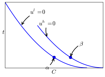
First, we replicate the figure in the exercise. An indifference curve in \((C,t)\) space takes the form \(u = t -\psi(e) = \bar u\) for some value \(\bar u \geq 0\). Hence, we get \(t = \bar u + \psi(\beta - C)\). We draw these indifference curves for \(\bar u =0\); that is, the curves correspond to the IR constraints.
The first best contract features \(e^*\) that minimizes total costs \(\beta - e + \psi(e)\): \(\psi'(e^*) = 1\). Hence, we have \(\psi'(\beta-C)=1\). With the quadratic \(\psi\) function that we have chosen, this yields \(\beta - C =1\) or equivalently \(C = \beta -1\).
beta_h = 3
beta_l = 2.5

def psi(C,beta):
        return 0.5*(beta-C)**2

rangeCh = linspace(1.0,3,200)
rangeCl = linspace(0.0,2.5,200)
plt.clf()
plt.rcParams.update({'axes.labelsize': 20,'text.fontsize': 20, 'legend.fontsize': 20})
plt.xlabel(r"$C$",fontsize = 20)
plt.ylabel(r"$t$",fontsize = 20,rotation = 0)
IRh = [psi(C,beta_h) for C in rangeCh] # this plots the indifference curve t = psi(beta-C) for beta^h
IRl = [psi(C,beta_l) for C in rangeCl] # here the indifference curve for beta^l
plt.plot(rangeCh,IRh,'-', color = 'b', linewidth = 2)
plt.plot(rangeCl,IRl,'-', color = 'b', linewidth = 2)
plt.xticks((),[]) # we don't need "ticks" on the axes
plt.yticks((),[])
alpha_point = plt.plot(1.5,psi(1.5,beta_l), 'ro') # here we mark the first best contract for beta^l on the IR constraint
plt.setp(alpha_point, 'markersize', 10)           # C = 2.5 - 1 = 1.5
plt.setp(alpha_point, 'markerfacecolor', 'b')
beta_point = plt.plot(2,psi(2,beta_h), 'ro')      # and for beta^h: C = 3 - 1 = 2
plt.setp(beta_point, 'markersize', 10)
plt.setp(beta_point, 'markerfacecolor', 'b')


plt.annotate('$\\alpha$', xy=(1.5,psi(1.5,beta_l)),  xycoords='data', # here we define the labels and arrows in the graph
              xytext=(-30, -40), textcoords='offset points', size = 20,
              arrowprops=dict(arrowstyle="->", linewidth = 2,
                              connectionstyle="arc3,rad=.2"),
              )
plt.annotate('$u^l = 0$', xy=(0.5,psi(0.5,beta_l)),  xycoords='data',
              xytext=(30, 40), textcoords='offset points', size = 20,
              arrowprops=dict(arrowstyle="->", linewidth = 2,
                              connectionstyle="arc3,rad=.2"),
              )
plt.annotate('$\\beta$', xy=(2, psi(2,beta_h)),  xycoords='data',
              xytext=(30, 40), textcoords='offset points', size = 20,
              arrowprops=dict(arrowstyle="->", linewidth = 2,
                              connectionstyle="arc3,rad=.2"),
              )
plt.annotate('$u^h = 0$', xy=(1.3, psi(1.3,beta_h)),  xycoords='data',
              xytext=(-30, 40), textcoords='offset points', size = 20,
              arrowprops=dict(arrowstyle="->", linewidth = 2,
                              connectionstyle="arc3,rad=.2"),
              )
plt.savefig('Regulation_fig1.png')
a Indifference curves are of the form \(t = \bar u - \psi(\beta - C)\). Hence,
because \(\psi' > 0\). In words, indifference curves are downward sloping.
To see how steepness varies with \(\beta\), we consider the second derivative:
because \(\psi'' >0\). Hence, higher \(\beta\) curves are steeper (have a “more negative slope”).
In the first best contract we have \(\psi'(\beta -C)=1\). As \(\beta\) increases, \(C\) must increase as well to keep \(\beta -C\) constant. Hence \(C\) is higher for \(\beta^h\) than for \(\beta^l\).
b The slope is given by \(dt/dC = -\psi'(\beta-C) = -1\) in first best as \(\psi'(\beta-C)=1\) in first best.
c Suppose contracts \(\alpha, \beta\) would be implemented under asymmetric information. Then \(\beta^l\) can raise her utility by choosing the “wrong” contract \(\beta\). This contract lies to the north east of her own contract \(\alpha\): higher \(t\) and higher \(C\) (and thus lower effort \(e\)) which is prefered by \(\beta^l\).
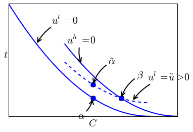
d To implement first best effort and cost levels while keeping the contracts IC, we need to raise \(t^l\) such that
where \(t^h = \psi(\beta^h - C^h)\) and hence the right hand side is strictly positive.
This leads to a new contract \(\tilde \alpha\) which gives type \(\beta^l\) strictly positive utility \(\tilde u >0\).
Note that contract \(\tilde \alpha\) lies to the south-west of \(\beta^h\)’s indifference curve. Hence \(\beta^h\) has no incentive to choose \(\tilde \alpha\) (“mimic \(\beta^l\)”).
The dotted line gives \(\beta^l\)’s indifference curve through the new contract \(\tilde \alpha\).
Summarizing, with contracts \(\tilde \alpha, \beta\), the planner can implement first best.
plt.clf()
plt.rcParams.update({'axes.labelsize': 20,'text.fontsize': 20, 'legend.fontsize': 20})
plt.xlabel(r"$C$",fontsize = 20)
plt.ylabel(r"$t$",fontsize = 20,rotation = 0)
IRh = [psi(C,beta_h) for C in rangeCh]
IRl = [psi(C,beta_l) for C in rangeCl]
rangeICl = linspace(1.0,2.5,200)
ICl = [psi(C,beta_l)+3.0/8.0 for C in rangeICl]
plt.plot(rangeCh,IRh,'-', color = 'b', linewidth = 2)
plt.plot(rangeCl,IRl,'-', color = 'b', linewidth = 2)
plt.plot(rangeICl,ICl,'--', color = 'b', linewidth = 2) # line style '--' draws a dashed line
plt.xticks((),[])
plt.yticks((),[])
alpha_point0 = plt.plot(1.5,psi(1.5,beta_l), 'ro')
plt.setp(alpha_point0, 'markersize', 10)
plt.setp(alpha_point0, 'markerfacecolor', 'b')
alpha_point = plt.plot(1.5,psi(1.5,beta_l)+3.0/8.0, 'ro')
plt.setp(alpha_point, 'markersize', 10)
plt.setp(alpha_point, 'markerfacecolor', 'b')
beta_point = plt.plot(2,psi(2,beta_h), 'ro')
plt.setp(beta_point, 'markersize', 10)
plt.setp(beta_point, 'markerfacecolor', 'b')


plt.annotate('$\\alpha$', xy=(1.5,psi(1.5,beta_l)),  xycoords='data',
              xytext=(-30, -40), textcoords='offset points', size = 20,
              arrowprops=dict(arrowstyle="->", linewidth = 2,
                              connectionstyle="arc3,rad=.2"),
              )
plt.annotate('$\\tilde{\\alpha}$', xy=(1.5,psi(1.5,beta_l)+3.0/8.0),  xycoords='data',
              xytext=(+30, +40), textcoords='offset points', size = 20,
              arrowprops=dict(arrowstyle="->", linewidth = 2,
                              connectionstyle="arc3,rad=.2"),
              )
plt.annotate('$u^l = 0$', xy=(0.5,psi(0.5,beta_l)),  xycoords='data',
              xytext=(30, 40), textcoords='offset points', size = 20,
              arrowprops=dict(arrowstyle="->", linewidth = 2,
                              connectionstyle="arc3,rad=.2"),
              )
plt.annotate('$u^l = \\tilde u>0$', xy=(2.2,psi(2.2,beta_l)+3.0/8.0),  xycoords='data',
              xytext=(30, 40), textcoords='offset points', size = 20,
              arrowprops=dict(arrowstyle="->", linewidth = 2,
                              connectionstyle="arc3,rad=.2"),
              )
plt.annotate('$\\beta$', xy=(2, psi(2,beta_h)),  xycoords='data',
              xytext=(30, 40), textcoords='offset points', size = 20,
              arrowprops=dict(arrowstyle="->", linewidth = 2,
                              connectionstyle="arc3,rad=.2"),
              )
plt.annotate('$u^h = 0$', xy=(1.3, psi(1.3,beta_h)),  xycoords='data',
              xytext=(-30, 40), textcoords='offset points', size = 20,
              arrowprops=dict(arrowstyle="->", linewidth = 2,
                              connectionstyle="arc3,rad=.2"),
              )
plt.savefig('Regulation_fig2.png')
e Implementing first best is only optimal if \(\lambda =0\). That is, the planner does not worry about paying high rents (\(\tilde u >0\)) to \(\beta^l\). If \(\lambda > 0\), it becomes optimal to distort \(\beta^h\)’s contract.
This can be seen as follows. By distorting \(\beta^h\)’s contract, we reduce welfare, but this is a second order effect (as we start from first best). By distorting this contract, we can reduce the rents we pay to \(\beta^l\) which is a first order gain for \(\lambda >0\).
f Start from the first best contracts. Reduce the rents that the planner pays to \(\beta^l\) by moving \(\beta^l\)’s indifference curve downwards. This implies that \(\beta^h\)’s contract moves to the right and downward; i.e. it gets distorted with inefficiently high costs \(C\) (due to inefficiently low effort \(e\)). By doing this, we reduce rents, without giving \(\beta^l\) an incentive to mimic \(\beta^h\). We keep \(\beta^h\) on her IR constraint.
The trade off is: the further we reduce the rents paid to \(\beta^l\) (move \(\beta^l\)’s indifference curve downwards), the more we have distort \(\beta^h\)’s effort and costs.
g See figure below with second best contracts \(\hat \alpha, \hat \beta\).
plt.clf()
plt.rcParams.update({'axes.labelsize': 20,'text.fontsize': 20, 'legend.fontsize': 20})
plt.xlabel(r"$C$",fontsize = 20)
plt.ylabel(r"$t$",fontsize = 20,rotation = 0)
IRh = [psi(C,beta_h) for C in rangeCh]
IRl = [psi(C,beta_l) for C in rangeCl]
rangeICl = linspace(1.0,2.5,200)
ICl = [psi(C,beta_l)+3.0/8.0 for C in rangeICl]
ICl2 = [psi(C,beta_l)+3.0/16.0 for C in rangeICl]
plt.plot(rangeCh,IRh,'-', color = 'b', linewidth = 2)
plt.plot(rangeCl,IRl,'-', color = 'b', linewidth = 2)
plt.plot(rangeICl,ICl,'--', color = 'b', linewidth = 2)
plt.plot(rangeICl,ICl2,'--', color = 'r', linewidth = 2)
plt.xticks((),[])
plt.yticks((),[])
alpha_point0 = plt.plot(1.5,psi(1.5,beta_l), 'ro')
plt.setp(alpha_point0, 'markersize', 10)
plt.setp(alpha_point0, 'markerfacecolor', 'b')
alpha_point = plt.plot(1.5,psi(1.5,beta_l)+3.0/8.0, 'ro')
plt.setp(alpha_point, 'markersize', 10)
plt.setp(alpha_point, 'markerfacecolor', 'b')
alpha_point1 = plt.plot(1.5,psi(1.5,beta_l)+3.0/16.0, 'ro')
plt.setp(alpha_point1, 'markersize', 10)
plt.setp(alpha_point1, 'markerfacecolor', 'r')
beta_point = plt.plot(2,psi(2,beta_h), 'ro')
plt.setp(beta_point, 'markersize', 10)
plt.setp(beta_point, 'markerfacecolor', 'b')
C_l = optimize.root(lambda x: psi(x,beta_l)+3.0/16.0-psi(x,beta_h) , 2.5).x[0]
beta_point2 = plt.plot(C_l,psi(C_l,beta_h), 'ro')
plt.setp(beta_point2, 'markersize', 10)
plt.setp(beta_point2, 'markerfacecolor', 'r')


plt.annotate('$\\hat{\\alpha}$', xy=(1.5,psi(1.5,beta_l)+3.0/16.0),  xycoords='data',
              xytext=(-50, -40), textcoords='offset points', size = 20,
              arrowprops=dict(arrowstyle="->", linewidth = 2,
                              connectionstyle="arc3,rad=.2"),
              )
plt.annotate('$u^l = 0$', xy=(0.5,psi(0.5,beta_l)),  xycoords='data',
              xytext=(30, 40), textcoords='offset points', size = 20,
              arrowprops=dict(arrowstyle="->", linewidth = 2,
                              connectionstyle="arc3,rad=.2"),
              )
plt.annotate('$\\hat{\\beta}$', xy=(C_l, psi(C_l,beta_h)),  xycoords='data',
              xytext=(30, 40), textcoords='offset points', size = 20,
              arrowprops=dict(arrowstyle="->", linewidth = 2,
                              connectionstyle="arc3,rad=.2"),
              )
plt.annotate('$u^h = 0$', xy=(1.3, psi(1.3,beta_h)),  xycoords='data',
              xytext=(-30, 40), textcoords='offset points', size = 20,
              arrowprops=dict(arrowstyle="->", linewidth = 2,
                              connectionstyle="arc3,rad=.2"),
              )
plt.savefig('Regulation_fig3.png')
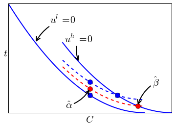
h We keep \(\beta^h\) on her IR constraint and hence \(IR_h\) is binding. \(\beta^l\) receives a rent and hence \(IR_l\) is not binding.
We want to avoid that \(\beta^l\) mimics \(\beta^h\) and hence \(IC_l\) is binding. Further, \(\beta^h\) strictly prefers contract \(\hat \beta\) above \(\hat \alpha\) (\(\hat \alpha\) lies below the indifference curve \(u^h = 0\)); hence \(IC_h\) is not binding.
i The second best contracts are determined by the trade off between the rents paid to \(\beta^l\) and the distorted effort of \(\beta^h\). As the probability \(\nu\) that a firm is \(\beta^l\) increases, the rents become more important (in expected welfare) compared to \(\beta^h\)’s distortion.
Hence, in response to an increase in \(\nu\), it is optimal to push \(\beta^l\)’s indifference curve downwards. This pushes contract \(\hat \beta\) to the right, raising \(C^h\).
Thus, the planner reduces \(\beta^l\)’s rents (\(t^l\) falls, while \(C^l\) is unchanged) and increases \(\beta^h\)’s effort distortion.